What is Symbulator

Symbulator is a program to solve linear electric circuits symbolically and numerically in a calculator. It accepts inputs with numerical and symbolic values, and provides numerical and symbolic results. The name is a portmanteau of "symbolic circuit simulator". Symbulator is widely regarded as the best symbolic simulator of linear electric circuits ever made for a calculator.

What analyses can it do?

Symbulator can perform direct current (DC) analysis, alternating current (AC) analysis (as phasor analysis), transient time-domain (TR) analysis, and complex frequency-domain (FD) analysis.

Symbulator can analyse numerical and, more importantly, symbolic linear circuits. It will return the voltages in all nodes, and the currents, voltage drops and power in all elements.

Symbulator can also find the Thévenin, Norton and two-port equivalent of a circuit. It can do time domain and Bode plots.

What elements does it accept?

Symbulator accepts elements such as resistors, inductors, mutual inductance, capacitors, independent and dependent current and voltage sources, ideal operational amplifiers, ideal transformers and six types of two-ports.

Where does it run?

Symbulator 8 has been adapted to run on the TI-Nspire CX II CAS calculator by Texas Instrument. There is also a version for the TI-89 Titanium, called version 7.

Why use Symbulator?

Symbulator is extremely useful in solving a wide variety of circuits theory problems, such as those taken by engineering students in Circuits I and Circuits II classes. It allows the student to focus on the conceptual understanding of circuit analysis, rather than the mathematical techniques used for their solution.

Strengths

Symbulator is a fantastic tool when you need a symbolic approach to solve small or medium sized circuit composed of ideal, linear elements.

You can use Symbulator whenever you have to solve circuits with symbolic values or when you need symbolic results.

When compared to PSpice or MultiSim, this small software offers a simpler way to define dependent sources, and includes special elements such as ideal transformers and six different two-ports, usually not included in other simulators.

Limitations

Since it is a linear circuit simulator, Symbulator does not simulate non-linear elements, such as diodes and transistors.

Symbulator is not a replacement for your brain or an excuse to not study your circuit theory classes: you must understand circuits theory to use it.

Finally, Symbulator will not help you answer problems that rely on applying formulas selectively, as opposed to solving a circuit completely.

Symbulator is free!

You do not have to pay anything to use Symbulator. It has always been free of cost, and always will be. (You are welcome!)

Since June 2013, Symbulator is offered under a Creative Commons License (CC) BY-NC-SA. If you want to port it to other platforms, you are free to do so under the same license.

Furthermore, I'm currently working with my friend Qifan Wang to convert Symbulator into an open-source program that runs on an open-source CAS. More on that soon.

Download

Symbulator

The version of Symbulator for the TI-Nspire CX II CAS is called version 8 alpha (date stamp 08 July 2023). It may still contain bugs. Do not use it for anything important yet. As bugs are discovered and fixed, we will revise and reupload the program, updating the date stamp above. Version 8 is an adaptation of Version 7, the final version of Symbulator for the TI-89 platform (including TI-89 Titanium and the Voyage 200).

To get Symbulator 8, download this file: s.tns, transfer it to your TI-Nspire CX II CAS, and refresh the libraries.

If you have any problems downloading, installing or executing Symbulator, send us a message to this email: the word help at this domain. Like this: help@sxxxxxxxxx.com

Laplace Functions

Since the CAS in the TI-Nspire CX II CAS calculator does not do Laplace transforms, Symbulator relies for this on another software. I call this software Laplace Function.

A bit of history

This Laplace software was made, around the same time as Symbulator was being created, by my friend Lars Frederiksen, one of the most gifted programmers for TI-Basic ever. Lars made two programs for Laplace for the TI-92+/Voyage and the TI-89: one he called DiffEq, a reference to the fact that it also solves differential equations, and the other one called Advanced Laplace, which packed improved version of his Laplace functions.

The latter software was automatically adapted for the TI-Nspire by Philippe Fortin, who renamed the group of functions as ETS_specfunc. This specfunc program has been popularised by the tutorials of Michel Beaudin.

I am a big fan of Lars's work on Laplace. Actually, for many years I hosted his programs exclusively on my website, at his request, and had the honor of helping him beta-test them for the TI-89.

Since I am not a fan of the new name assigned to this program at the time of porting, and given my friendship and collaboration with Lars in the past, I have taken the liberty of renaming the file here to LF, which in my eyes stands both for Laplace Functions and for Lars Frederiksen, in homage to the author of this brilliant piece of code. You need to download this file: lf.tns, transfer it to your calculator, and refresh the libraries.

Solved Problems

I have solved all the problems in this documentation, each in a separate document in the format of the TI-Nspire. This zip file: problems.zip contains three hundred solved problems.

Before you start

Clean slate

I recommend that, before running a simulation in the Nspire, you either create a new document, or delete all the variables that are not related to your simulation from the current document.

Furthermore, if for any reason a simulation fails or aborts and there are leftover variables, you should either move to a new document or delete these variables before you run the simulation again.

Direct current analysis

I want you to create a new document in your calculator, or to delete all variables you don't need from your current one (ideally, the current document should be empty), and type this:

s\dc("e1,1,0,36:r1,1,2,1'k:r2,2,3,3'k:r3,3,0,2'k")

Now I want you to press ENTER.

If you typed everything correctly, and your calculator is properly set up with Symbulator, you should have seen several lines of text appear on the screen, with a series of cryptic messages. Then, after a few seconds, it should have displayed a short message of Done.

You have just run your first simulation in Symbulator. Congratulations!

Deconstructing the spell

Let's now go over what exactly it is that you typed, one piece at a time.

To analyze a direct current circuit in Symbulator, we use a program called s\dc(). The program itself is called dc, but since it is found in the Symbulator library s, we have to refer to it as s\dc), so the calculator knows exactly what we want. And because it is a program, it carries the parenthesis () after its name.

The dc program takes one argument as its input: the description of the circuit you want to analyze. That input goes inside the parenthesis.

In Symbulator 8, a circuit description takes the form of a string of text, describing a series of elements, separated by colons.

The circuit description can be passed to the program directly as an argument when you invoke the program, as we did above, or it can be stored into a variable whose name is then fed into the program as an argument, like this:

"e1,1,0,36:r1,1,2,1'k:r2,2,3,3'k:r3,3,0,2'k"→cir

You can use any allowable variable name to store your circuit. I like to use cir as the name of the variable where I store my circuits, and that's what you will see in this tutorial. But you are free to use any other valid variable name.

Once we have stored the circuit description string into a variable, we can call the dc program, giving it that variable name as its input, like this:

s\dc(cir)

In terms of the simulation, the results of doing it this way are exactly the same as doing it in a single step. Throughout this text, you will see both ways being used.

Look at the elements

Now let's examine the contents of the circuit description, that is, the contents of the string. Study it, and you will see that there are three colons in it. In Symbulator, colons are used to separate elements in a circuit description. Thus, putting the colons aside, we can see that in this description there are four elements being described:

• The first one is e1,1,0,36
• the second one is r1,1,2,1'k
• the third one is r2,2,3,3'k and
• the fourth one is r3,3,0,2'k

At the moment, they may look cryptic and indecipherable. But by the time you are done with this lesson, you will be able to understand them with ease.

How to describe a resistor

Notice that the second, third and fourth elements in the list all start with the letter r. These are resistors.

For example, an ideal resistor called r1, connected between two nodes called a and b with a resistance of 300 Ω, would be described in Symbulator as follows: r1,a,b,300

How to name resistors

Every resistor in your circuit must have a name. As long as it starts with the letter r, and as long as it is unique, this name can be whatever you want. There are two exceptions I know of so far: the names r and rr should not be used as names for resistors, because some of the variables they generate as answers have the same name as reserved variables.

How to name nodes

As you know, naming the nodes in a circuit is probably the first things we all do before we analyze it. In a circuit description for Symbulator, every node in your circuit must have a name. Node names must be unique: no other node or circuit element should have the same name. As long as these names are unique, they can be whatever you want, with two constraints. The first one is that at least one node should be called 0 (zero). This will be considered the ground node of your circuit and will have, by definition, a voltage of 0 volts.

The second restriction is that you cannot use variables that are reserved in the calculator as names. These are listed in the User's Manual of the calculator.

Values can use SI prefixes

The values of circuit elements are often given using prefixes of the International System (SI), such as kilo, mili, micro, etc. Because of this, Symbulator includes a shorthand that helps it understand SI prefixes. Whenever a SI prefix is used in the value of an element, preceded by an apostrophe, in the circuit description or other inputs passed to the program, Symbulator will multiply it by the corresponding factor, using exact values.

So, for example, the value of a 3k Ω resistor can be described to Symbulator as 3'k, and it will understand that this means 3x10^3 (e.g., 3 times a thousand). The value of 8k Ω resistor can be entered in many ways: 8000, 8'k,8000. and 8E3 are all equivalent, except that the first two will be treated by the calculator as exact values, while the other two will be treated as approximate values.

What answers do you get

After the simulation in DC is complete, Symbulator stores a series of answers in the calculator's memory, labeled with easy to remember names for your convenience.

Answer for each node

For each node used in the description of the circuit, its voltage with reference to the ground is stored in a variable called v plus the name of the node. For example, for a node called 1, its voltage with reference to ground is calculated and stored in a variable called v1.

Answers for each resistor

For each resistor included in the description of the circuit, the following answers are calculated and stored in the memory:

• The voltage drop in the resistor, that is to say, the voltage in the first node declared minus the voltage in the second node declared, is stored in a variable called v plus the name of the resistor. This value is in volts. For example, for a resistor called r5, the voltage drop is stored in vr5.
• The current through the resistor, flowing from the first node towards the second, is stored in a variable called i and the name of the resistor. This value is in amperes. For example, the current flowing through resistor rx, from the first node declared towards the second node declared, is stored in irx.
• The power consumed by the resistor is stored in a variable called p and the name of the resistor. This value is in watts. For example, the power consumed by resistor r12 is stored in pr12.

By now, you should be able to understand the description of the second, third and fourth elements in our example.

How to describe a voltage source

The first element in our example, on the other hand, started with the letter e. This element is a voltage source.

For example, an ideal voltage source called e1, connected with its positive terminal in node 3 and with its negative terminal in the ground node 0, with a value of 12 volts (understood as the voltage of the positive node with regards to the negative node), would be described in Symbulator as follows: e1,3,0,12

How to name voltage sources

Every voltage source in your circuit must have a unique name that starts with the letter e, and it can be whatever you want.

Values can use SI prefixes

The values of a voltage source in the circuit description can also use SI prefixes. They can be used in the values of all element in the circuit description.

So, that's how you describe a voltage source.

Answers for a voltage source

For each voltage source included in the description of the circuit, the following answers are calculated and stored in the memory:

• The voltage drop in the source, that is to say, the voltage in the first node declared minus the voltage in the second node declared, is stored in a variable called v plus the name of the source. This value is in volts. For example, for a source called e5, the voltage drop is stored in ve5.
• The current through the source, flowing from the first node towards the second, is stored in a variable called i and the name of the source. This value is in amperes. For example, the current flowing through source ex, from the first node declared towards the second node declared, is stored in iex.
• The power consumed (attention: not delivered, but consumed) by the source is stored in a variable called p and the name of the source. This value is in watts. For example, the power consumed by a source e12 is stored in pe12. If we want the power delivered, we ask for the negative of this value, namely –pe12 (where "–" is the negate symbol, not to be confused with "-" the subtract symbol).
• The equivalent resistance of the rest of the circuit, as seen by the source, is stored in a variable called r and the name of the source. For example, the equivalent resistance of a circuit as seen from a source called e2 is stored in variable re2.

A numerical DC simulation, step by step

Let's go back now to the simulation we ran earlier. That simulation corresponds to the circuit given in Example 5.7 in Boylestad’s Introductory Circuit Analysis (11ed). Moving forward, I will refer to that textbook as B11. For your benefit, the problem statement and the circuit schematic have been scanned and are reproduced below, exactly as they appear in the textbook. This will be the case in every other problem shown in this tutorial. Since this is for educational purposes, e.g., to teach you how to use Symbulator, it is my understanding that it falls squarely within the "fair use" doctrine of copyright law. In any event, no copyright infringement is meant. Ok, here we go.

As you can see, all the values in this circuit are numbers, e.g., no element values are unknown. This is an example of a numerical circuit. A circuit is numerical if we know the numerical value of every element in the circuit.

I will now walk you step by step through the solution of this numerical problem in Symbulator 8. The process you will see here applies to most numerical simulations in Symbulator. First, you describe the circuit. Then, you run the simulation. Finally, you get the answers.

Step 1: Describe the circuit

The first step in solving a circuit is to describe it. Circuit description starts with naming the nodes. As we mentioned earlier, you can call the nodes anything you want, be it a number or a letter, as long as the name is unique. But you must always have one node called 0 (zero); this is your ground node and has a voltage of 0V. In this particular circuit, the ground node is indicated with the ground symbol, but that is not always the case. When it is not marked, you pick a node to serve as zero.

I labeled the nodes in this circuit, starting in the ground and moving clockwise, as 0, 1, 2 and 3. It helps me to pencil the names in the schematic itself.

After naming the nodes, I am ready to describe the elements of the circuit in Symbulator notation.

Let's start with the source: when I only have one voltage source, like here, I enjoy naming it with a single letter: e. Having chosen a name for it, I can now describe the voltage source as follows: e,1,0,36, given that its name is e, its positive node is called 1, its negative node is called 0, and its value is 36 volts between these nodes in that order.

Now I describe the resistors. I named the first resistor r1, and I described it as follows: r1,1,2,1'k, because it's name is r1, its first node is called 1, its second node is called 2, and its value is 1 kΩ. The second resistor we describe similarly: r2,2,3,3'k and likewise for the third resistor: r3,3,0,2'k.

Note: An important point regarding how to use SI prefixes is that, in the case of kilo, we can write it as either 'k or 'K. But that's not the case for every other SI prefix: their case matters. For example, 'm means mili, while 'M means mega. Symbulator's custom menu includes the spelling of all SI prefixes.

We pass the description of a circuit to Symbulator as a string. This means we open with a quotation mark, then enter the descriptions of each element as above, separated with colons, and then close with a quotation mark. We can store this string in a variable, like this:

"e1,1,0,36:r1,1,2,1'k:r2,2,3,3'k:r3,3,0,2'k"→cir

As I mentioned earlier, I like to call this variable cir (short for circuit,) but you can call it something else if you prefer. Once I press enter, the circuit will be stored in that variable and we are ready for the next step.

Step 2: Run the simulation

We can now ask Symbulator to simulate this circuit in direct current (DC), by typing this instruction in the calculator:

s\dc(cir)

And we press ENTER. Symbulator will now quickly solve in DC the circuit stored in the variable called cir. (As a reminder, another way to do this was to invoke the program and include the full string of the description in the parenthesis, like we did at the beginning of this lesson.)

Symbulator will let you know when it has completed a successful simulation by saying Done. It took my calculator under 2 seconds to solve this circuit. In that time, Symbulator found a total of 16 answers for this circuit, and stored each one in a memorably named variable in the current folder. For a DC analysis, these answers are as follows:

• The voltage of each node is stored in a variable called v plus the name of the node. So, the voltage of nodes 1, 2 and 3 are stored three variables called v1, v2 and v3.
• The current through each element is stored in a variable called i plus the name of the element. So, the current through resistor r1 is stored in a variable called ir1, and so on. An important point is that the direction of the current is defined as going from the first node in the element's description to the second node in the element's description.
• The voltage drop in each element is stored in a variable called v plus the name of the element. So, the voltage drop in resistor r1 is stored in a variable called vr1, and so on. An important point is that this voltage drop is defined as the difference in voltage between the first node in the element's description and the second node in the element's description, in that order.
• The power consumed in each element is stored in a variable called p plus the name of the element. So, the power consumed in resistor r1 is stored in a variable called pr1, and so on. An important point is that this is the power consumed, not the power delivered.
• Finally, for each source we get the equivalent resistance of the rest of the circuit as seen by that source. This is stored in a variable called r plus the name of the source. So, the equivalent resistance of the rest of the circuit as seen by the source called e is stored in a variable called re.

For this circuit, that amounts to 16 answers, solved and saved in 2 seconds. Not bad for a tiny program running on a calculator!

Step 3: Get the answers

With all of these values stored in the current folder, we can now get the answers we need for the six questions in the problem.

Answer to question (a): The equivalent resistance as seen by the source e is stored in a variable called re. Evaluating this variable returns the right answer: 6000 (that is to say, 6K Ω).

Answer to question (b): Current Is is defined in the schematic as the current flowing through the source, in the direction that goes from node 0 to node 1. One way to find this value is evaluating –ie (that is to say, the negative of the value stored in the variable called ie, which as you know contains the current flowing through the source from node 1 to node 0, that is to say, in the opposite direction as that requested in the question). Another way to find the answer, given that this is a series circuit where all elements have the same current through them, is to evaluate the current through any of the resistors: ir1, ir2 or ir3. In either case, the calculator provides the right answer: .006 (that is to say, 6mA).

Answer to question (c): The voltage drop in resistor R1 (since its polarity is defined in the schematic in the same way it is defined in our circuit description, namely node 1 as positive and node 2 as negative) can be found evaluating the value of variable vr1: the calculator returns 6 (e.g. 6 V.) For R2, we evaluate vr2 to obtain 18 V. And for R3, vr3 gives us 12 V. These are all the right answers.

Answer to question (d): Since the problem asks for the power supplied by the source, and we know that variable pe has the power consumed by it, we need to evaluate –pe (that is to say, the negative of the power consumed in source e) and we get the right answer: .216 (e.g. 216 mW delivered).

Answer to question (e): The power consumed by the resistors are found evaluating pr1, pr2, and pr3. The calculator returns the right answers: .036 (e.g. 36 mW), .108 (e.g. 108 mW), and .072 (e.g. 72 mW) consumed, respectively.

Answer to question (f): Let’s ask the calculator if the sum of the consumed power in the resistors equals the power supplied by the source. We evaluate this equation:

pr1+pr2+pr3=–pe

The calculator returns true. This is the right answer, and concludes the solution to this, your first ever problem in Symbulator.

Instructive numerical examples, solved

We have prepared a series of solved problems, involving numerical circuits that are composed solely of resistors and direct current voltage sources. Practicing these problems will help you assimilate better what you have learned so far, before moving to the next lesson. You can download them in a PDF by clicking here.

About symbolic problems

The problem we saw in Lesson 1 was a numerical problem because it involved a numerical circuit: from the start, we knew the numerical values for all the elements in it. None of them were unknown.

When a circuit has one or more elements for which we do not have a numerical value, we call it a symbolic circuit. A symbolic problem is one that involves a symbolic circuit. It gives me great joy when I encounter a symbolic problem, because the ability to simulate symbolic circuits is what sets Symbulator apart from other programs.

I find it useful to distinguish between two types of symbolic problems:

• Purely symbolic problems are problems that use symbolic circuits (e.g. circuits with unknown values) where the desired answers are also symbolic. In purely symbolic problems, the answers are given as expressions of unknown variables. Solving purely symbolic problems in Symbulator is as straightforward as solving numerical problems.
• Numerical-from-symbolic problems are problems that start with a symbolic circuit, but where we are asked to find numerical answers. Obtaining numerical answers starting from a circuit that contains unknown values is possible when the problem gives us additional information about the circuit. Numerical-from-symbolic problems can be solved in Symbulator in two ways:
  • If they are simple, e.g., if there’s just one or two unknown values in the circuit, and we are only asked for one or two numerical answers, then it is time-efficient to simulate the circuit symbolically and after that solve for the numerical answers, e.g., using the solve command of the calculator.
  • If they are not simple, e.g., if there are many unknown values in the circuit, or if we are asked to calculate many numerical answers, it is easier and more time-efficient to use the expert mode of Symbulator. We will introduce it to you later in this lesson.

Let’s see an example of each.

Solving a purely symbolic problem

Since Symbulator is natively a symbolic simulator, there is nothing special to solving a purely symbolic problem. The only limitation comes from the computing capacity of the calculator: while small circuits can be solved relatively fast, larger circuits may be too slow to solve and may cause a memory error (when the calculator runs out of memory to perform the computation that is required). Let's see a simple purely symbolic problem, from Fundamentals of electric circuits by Alexander and Sadiku (5th edition), onwards referred to as [AS5].

As you can see, all the values in this circuit are variables: no element values are known. This is an example of a symbolic circuit. Imagine you are asked to find symbolic expressions for the current i, the voltage drop in R2, and the power consumed by R1 and R2. Since we are being asked to find symbolic answers from a symbolic circuit, this would be a purely symbolic problem, that can be solved in a straight forward manner in Symbulator, as long as it's not too big.

This is how I would describe this circuit.

First, I name the nodes. The node called a in the schematic, I will still call node a. The node called b in the schematic will serve as my ground node, so I call it node 0. And the node between the two resistors, I will call node c.

Then, we name the elements. I will name the source ev, and will call the resistors r1 and r2. Now I am ready to describe my circuit, and store that description in a variable. For the values of the elements, I will use variables. The value of the source will be v, and the values of the resistors will be r1 and r2. It is not a problem that the symbolic value is the same as the name of the element.

"ev,a,0,v:r1,a,c,r1:r2,c,0,r2"→cir

Now we can call the dc program, with cir as its argument:

s\dc(cir)

This simulation took 15 seconds in my calculator. To find the current i, we ask for ir1 or ir2. To find the voltage drop on r2, we ask for vr2.

To find the power consumed in r2, we ask for pr2. To find the power delivered by the source, we ask for the negative of pev.

It is this ability to simulate symbolically as if nothing that puts Symbulator in a league of its own. Getting symbolic answers from a symbolic circuit takes no extra effort.

Numerical from symbolic, with solve

Getting numerical answers from a symbolic circuit, on the other hand, requires an additional step. This additional step can be the use of the solve command of the calculator, as we will see in this next example. Or it can be the use of the expert mode, as we will see in the example after that.

This is a very nice numerical-from-symbolic problem. We should be able to solve it into numerical results because, even though the problem hides two values from us (e.g., the value of the source E and of the resistor R1), it gives us in exchange two answers (e.g., the equivalent resistance RT and the current I3) that we can use to solve for the unknowns.

Since this circuit is structurally identical to B11’s Example 5.7 solved in Lesson 1, we will use the same names for the nodes. The circuit description is identical except for the element’s values. As values for the elements in the circuit, Symbulator will accept numbers, variables or even algebraic expressions. For this example, I will use e for the value of source e, and r1 for the value of the r1 resistor.

Below is how I described this circuit. I pass along this description to Symbulator as a string, and store it in a variable called cir.

"e,1,0,e:r1,1,2,r1:r2,2,3,4'k:r3,3,0,6'k"→cir

Ask Symbulator to simulate this circuit in direct current:

s\dc(cir)

A moment later, Symbulator is done, and we are ready to answer the questions. Using the symbolic answers provided by Symbulator and the known answers given by the problem, we will write two equations. We will then solve these two equations for the two unknowns that interest us, using the calculator’s solve command. (If you are not familiar with the solve command, I refer you to the calculator’s manual.) Let’s explore what we have here.

The problem says that I3 is 6mA. In Symbulator, I3 is called ir3 (e.g. the current through resistor r3.). If you evaluate ir3, you will see it produces an algebraic expression in terms of the two unknowns, e and r1. This is what we call a symbolic answer. The problem also says that RT is 12K Ω. As we saw in the previous problem, the equivalent resistance as seen by the source e is given by re, which when evaluated gives another algebraic expression in terms of r1. We can then write two new equations, re=12000 and ir3=6/1000, and solve them for the two unknowns we want: e and r1.

solve(re=12000 and ir3=.006,{e,r1})

(Notice that you cannot use the 'k here as a shorthand for kilo, or any other SI prefixes, because that shorthand only works within the values in the description of the circuit.)

An instant later we get the answers: e = 72. V and r1 = 2000 Ω. These are the right answers. Not many other circuit simulators allow this flexibility.

Now let’s see what the the expert mode has to offer.

Numerical from a symbolic, using ex

Symbulator’s true strength is seen in numerical-from-symbolic problems like the one we solved above, when we use its expert mode of simulation. expert mode cracks these problems open even faster, and can give you fully numerical values to all the answers of problems like, e.g., problems that have an equal number of unknown values and of answers provided by the problem. Learning to use the expert mode pays off handsomely in terms of additional power and speed.

Let’s solve the same circuit again, this time using the expert mode's program ex.

We will use the same circuit description as before, with a single change: we will use rx for the value of resistor R1, instead of the r1 value we used before. Like this:

"e,1,0,e:r1,1,2,rx:r2,2,3,4'k:r3,3,0,6'k"→cir

We use rx instead of r1 for our symbolic value because the expert mode will try to save into that variable the value it finds, and r1 (as well as other r# variables) cannot be used to store anything: trying to store a value into r1 results in an error.

To run an expert mode simulation, type this in the calculator:

s\ex(cir)

When prompted, select DC and press Enter. Now you will see a prompt asking you to add equations, variables and conditions. You may recall from your algebra class that you need an equal number of equations and unknowns in order to solve a set of equations into numerical values. The statement of the problem gives us the information we need to write the two additional equations.

(We know the value for RT and the value for IS in terms of the variables listed in the prompt: because RT is given by re, which is a function of e and ie, and IS is given by ir3, which is a function of ie.)

In "Add equations" type:

re=12'k and ir3=6'm

In "Add unknowns" type:

e,rx

Now we have six variables and six equations. Press Enter and wait just a few seconds. A few of other dialogs will appear. In this and all the other Expert examples in this volume, just press OK in these prompts without changing anything in them. When Symbulator says "Done", go ahead and retrieve the answers:

rx

You get 2000, the right answer.

e

You get 72, the right answer.

The speed advantage of the expert mode is not necessarily evident in this simple problem. It does give you an idea of what the expert mode is all about: you get to halt the simulation in mid-air and give Symbulator extra information. Had this circuit been larger, the benefit of the expert mode in computation time would be clear.

Instructive symbolic examples, solved

We have prepared a series of solved problems, involving symbolic circuits that are composed solely of resistors and direct current voltage sources, with at least one unknown value. The examples include solutions using both solve and ex. Practicing these problems will help you assimilate better what you have learned so far, before moving to the next lesson. You can download them in a PDF by clicking here.

How to describe a current source

For example, an ideal current source called j1, connected between two nodes called 0 and 3, with a current of 5A running through, it from the first node to the second node, would be described in Symbulator as follows: j1,0,3,5

You can use SI prefixes here as well. The value of a current source is often given in milli-amps. Symbulator will interpret any 'm given in the value to means 3x10^-3 (e.g., 3 divided by a thousand).

Answers for a current source

For each current source included in the circuit description, you get the same answers you would get for a voltage source, using the same polarity conventions: the voltage drop in it, the current through it, the power consumed by it (for the delivered power, ask for the negative), and the equivalent resistance of the rest of the circuit as seen by that source.

Let's see an example.

Given the circuit below, determine the current and voltage drop in R1.

We ask Symbulator to run a DC simulation of the circuit described between quotations:

s\dc("j,0,1,10'm:r1,1,0,20'k")

We ask for the values of two variables: ir1 and vr1. The calculator returns .01 and 200. meaning a 10mA current and a 200V voltage drop.

What about conductaces?

Conductances are really resistors by another name. So, we describe them as resistors, using the element r, and we enter as the value the inverse of the conductance: one divided by the value of the conductance gives you the value of the resistor in Ω.

The following example is taken from the textbook Elementary Linear Circuit Analysis (2ed) by Leonard S. Bobrow. From this point forward, I will refer to this book as Bo2.

Given the circuit below, determine the voltages in the nodes.

As I explained before, in Symbulator all conductances are simulated as resistors. So, the 4 siemens conductance becomes a 1/4 resistor, and so on. Below my description:

s\dc("j10,1,0,2:r12,1,2,1:r20,2,0,1/4:r30,3,0,1/3:r13,1,3,1/2:j32,3,2,3")

We ask for these answers:

approx({v1,v2,v3})

The answer, {–1.3,.34,–1.12}, indicates v1=–1.3V, v2=.34V, v3=–1.12V. This is correct.

How to reduce parallel resistors

Symbulator has a way to help you reduce two resistors connected in parallel to their equivalent. It is a function called pr, and you can use it either on its own or as part of circuit descriptions. Furthermore, to save you some typing, you can invoke it on the fly using a shorthand as part of circuit descriptions.

Using s\pr({r,r,r...})

When you do not need to know the current through, or the power consumed by, each individual resistor, you can reduce the value of any number of resistors in parallel to their equivalent resistor value. You do this by invoking the s\pr function, and giving it as its input a list of resistance values that you want to reduce, separated by commas. This can be any number of values.

For example, say that you want to reduce three resistors in parallel with values of 10 Ω, 20 Ω and 30 Ω. You can do that by typing s\pr({10,20,30}). You get the answer of 60/11 if you evaluate exactly, or 5.45 if you evaluate approximately.

You can also give symbolic values for the resistances. For example, say that you want to reduce four resistors in parallel with values of r1, r2, r3 and r4. You can do that by typing s\pr({r1,r2,r3,r4}). You get the answer as a symbolic expression.

You can use the s\pr tool as part of a circuit description or on its own, on the entry line of the calculator, outside of Symbulator. This is useful because sometimes you may not even need to run a simulation to find the answer to a problem which is basicaly a resistor reduction problem.

Reducing series and parallel combos

A similar reduction of resistors in series is possible through simple addition whenever we do not need to know specific answers for each resistor, such as the voltage drop or power consumed in each, or the voltage in the node between them. The current through series resistors is the same, so even through an equivalent you can get the current.

Reducing a combination of series and parallel resistors is possible by a combination of addition and the use of the s\pr function. Let's see a couple of examples:

Find the equivalent resistance.

We don't need to run a simulation in Symbulator to find this answer. We can find it by typing this in the entry line of the calculator:

10+s\pr({3,6,1+s\pr({12,4,1+5})})

We evaluate approximately and get: 11.2 Ω. This is correct.

Find the equivalent resistance.

We don't need to run a simulation in Symbulator to find this answer. We can find it by typing this in the entry line of the calculator:

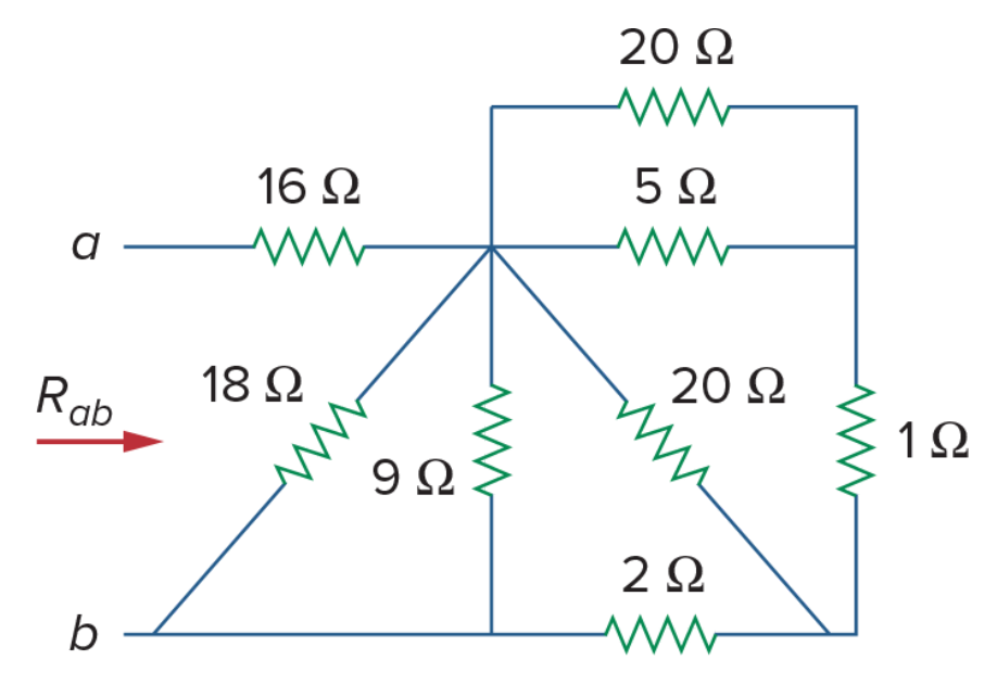
16+s\pr({18,9,2+s\pr({20,1+s\pr({5,20})})})

We evaluate and get: 19 Ω. This is correct.

The [r,r,r...] shorthand for descriptions

it may not be too practical to have to type s\pr({}) while you describe the circuit. So, to make it easier to call for the reduction of parallel resistors on the fly, as you type a circuit description, I have added a shorthand. Symbulator will recognise any values inside square brakets, such as these: [10,20,30] or these [r1,r2,r3,r4], as input to be passed to the s\pr function. This shorthand only works within the circuit description that is passed to Symbulator, and will not work outside of it.

When to reduce resistors

For example, a simulation where it makes sense to use pr is B11’s Example 7.4, which you saw in the practice problems of Lesson 1. It makes sense to reduce R4 and R5 to an equivalent resistor, since we do not need to know their individual currents or power use. So we can invoke s\pr:

s\dc("e,1,0,16.8:r1,1,2,9:r2,1,2,6:r3,2,3,4:re,3,0,[6,3]:r6,2,0,3")

An example of a simulation where using pr makes no sense is B11’s Example 8.3 (which you will see in the practice problems of Lesson 3). It makes no sense to reduce R1 and R2, because you need to know the value of the current through R1.

Finally, a simulation where you can reduce part of the resistors using pr is B11’s Example 6.22 (which you will see in the practice problems of Lesson 3). We must leave R1 alone, because we need to know the current through it, but we can reduce R2 and R3 to their equivalent using s\pr, since we do not need to know their individual currents or power use:

s\dc("jt,0,1,12'm:r1,1,0,1'k:re,1,0,[10'k,22'k]")

Moving forward, we will use the pr({,,}) tool, or its shorthand [,,], in circuit descriptions whenever we feel it is appropriate.

How to describe dependent sources

One of my favorite scenes in cinema comes from The Dark Knight: the Joker (played masterfully by Heath Ledger) is rolling on the floor of a Gotham City prison, taking a bare-knuckle beating from an ever-more-frustrated Batman. Master of the situation and laughing hysterically, the Joker says: "You have nothing! Nothing to threaten me with!"

Even though the movie had not been made yet, I remember feeling something along the same lines - although maybe less hysteric - back in 1999, when I realized that one of the consequences of having used a 100% symbolic implementation for Symbulator was that I could make any element’s value dependent on any answer of the circuit. I could simulate voltage or current sources that were dependent on any voltage, current or combination thereof, with the same ease that I could simulate a 12V source.

Here is what you need to know for simulating dependent sources on Symbulator: nothing. There is nothing special to it, nothing at all. Just write the value as a function of the circuit’s answers, using the variables that by now you should know well, and run the simulation like it’s nobody’s business. For example:

• if the source depends on the current through a resistor called r1, you define its value as ir1
• if the source depends on the voltage drop in resistor called r2, you define its value as vr2
• if the source depends on the current through a short called s3, you define its value as is3
• if the source depends on the difference between the voltage of two nodes a and b, you define its value as va-vb

With Symbulator, instead of fearing them, you will laugh in the face of dependent sources, thinking: "You have nothing!" Booyah!

In the solved problems for this Lesson, you will find plenty of examples with dependent sources of all types. Enjoy!

Instructive solved examples

We have prepared a series of solved problems, involving both numerical and symbolic DC circuits, composed solely of resistors (including as conductances) and of voltage and current sources (both dependent and independent). Practicing these problems will help you assimilate better what you have learned so far, before moving to the next lesson. You can download them in a PDF by clicking here.

How to describe a short circuit

Shorts are used mostly when we need to find out a current in a part of the circuit where there is no element already. Otherwise, we would just define it as a single node.

For example, an ideal short circuit called s1, connected between two nodes called 3 and 5, would be described in Symbulator as follows: s1,3,5

What answers do you get

No power is consumed, and no voltage is dropped in a short circuit. For each short in a circuit, Symbulator stores only the current through it, flowing from the first node towards the second, in a variable called i and the name of the short. For example, the current flowing through a short called sx, from the first to second node, is stored in isx.

Let's see an example.

Find i1, i2, i3 and i4.

My solution below. I define the shorts in the same direction as the arrows in the schematic.

s\dc("r1,1,0,25:jd,0,2,.2v1:r2,2,3,10:ji,4,3,2.5:r3,4,5,100:s1,1,2:s2,2,4:s3,0,3:s4,3,5")

We ask for the values of the variables:

approx({is1,is2,is3,is4})

The calculator returns the answers {–2.,3.,–8.,–.5}, which are correct. These answers can only be found using short circuits.

The equivalent resistance script: er

As we saw before, Symbulator has the ability to provide the equivalent resistance of a circuit as seen from any source. This allows us to solve problems like the following:

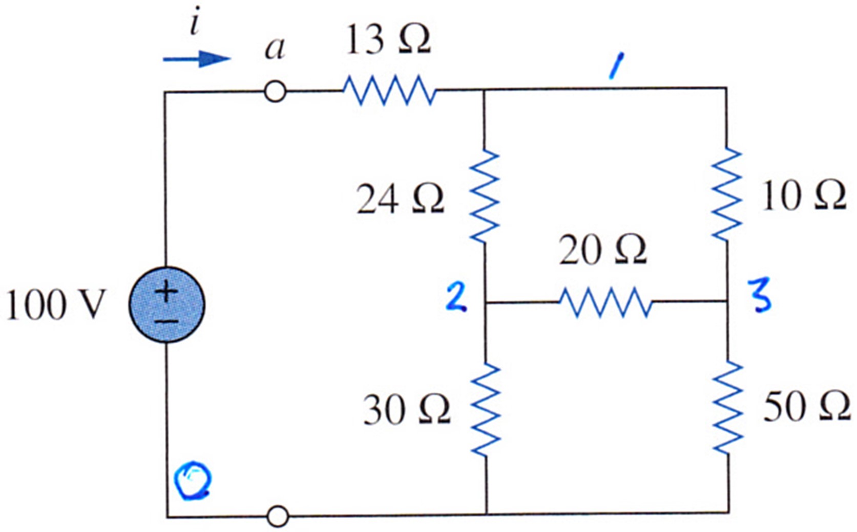
Find the equivalent resistance as seen by the 100V source, and the value of current i.

Below my solution:

s\dc("e,a,0,100:r13,a,1,13:r24,1,2,24:r10,1,3,10:r20,2,3,20:r30,2,0,30:r50,3,0,50"):re

By evaluating re we get the value of the equivalent resistance as seen by the source e. It is 40 Ω. By evaluating ir13 we get a value of 2.5A for current i. The answers were easily found, because there was a source connected between the two desired nodes.

What if there is no independent source?

But how can we find the equivalent resistance of a passive circuit, that is to say, a circuit that has no independent source in it? One way to find this in Symbulator is to connect a 1A current source between the two nodes where we want to find the equivalent resistance, and then read the voltage drop across the source. This is the manual way.

An easier way is to let Symbulator do that for us. Just run the er script, and it will do the same thing for you, automatically. The er script finds the equivalent resistance of a passive circuit, and stores it - in the case of a DC analysis - in a variable called req. The er script takes three arguments: the first is the circuit description in the form of a string; the second and third are the two nodes between which we need to find the equivalent resistance. Let’s learn by doing.

Calculate the equivalent resistance of the circuit shown below.

Let me solve this problem step by step. After I label the nodes, I describe the circuit. In this case, I store it in a variable.

"r4,0,a,4:r2,0,b,2:r6,a,b,6:rb,a,c,3:ra,b,c,3"→cir

Run the er script, giving it as arguments the circuit and the nodes:

s\er(cir,0,c)

When prompted, choose DC as analysis type. Once it is done, evaluate:

approx(req)

The value is 2.89 Ω. This is correct.

What counts as a passive

The example above was made of resistors only. The er script can be applied to a second type of passive circuits: circuit that include resistors and dependent sources, but no independent sources. A circuit with no independent sources can only be reduced to an equivalent resistance, not to a Thévenin or Norton equivalent, so the proper script to use is er. The script is used in exactly the same manner as for resistive circuits, making sure the dependent sources are described properly, according to the conventions of Symbulator notation. At the end of this session we offer you a series of examples of passive circuits, but purely resistive and with dependent sources, for you to practice.

The Thevenin / Norton script: th

Just like a passive circuit can be reduced to an equivalent resistance, an active circuit (e.g., one with independent sources) can be reduced to a Thévenin or Norton equivalent.

One way to find the Thévenin or Norton equivalent of an active circuit using Symbulator is to run a first simulation of the circuit to find out the voltage between the two nodes where we want to find the equivalent (this is the Thévenin voltage, or V_TH), and then to run a second simulation with a short-circuit connected between these two nodes to find out the circuit running through it (this is the Norton current, or I_NO). We can then get the equivalent resistance, or REQ, by dividing V_TH/I_NO. Notice that R_EQ is often called the Thévenin resistance. This is the manual way.

An easier way to find the Thévenin and Norton equivalent of a circuit in Symbulator is to run the th script, which does exactly the same thing described above, automatically.

The th script finds the Thévenin and Norton equivalents of an active circuit. It takes three arguments: the circuit description, the first node and the second node. Once you run it, the script finds and stores in the memory a series of useful answers, which we will discuss in a moment. Let's see an example:

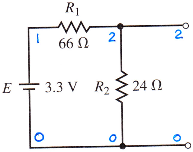
Find the Thévenin and Norton equivalents of the circuit below.

This is my circuit description:

"e,1,0,3.3:r1,1,2,66:r2,2,0,24"→cir

And this is how we run the tr script:

s\th(cir,2,0)

We could also have passed the circuit description directly like this:

s\th("e,1,0,3.3:r1,1,2,66:r2,2,0,24",2,0)

When prompted to select a type of analysis, choose DC. In the calculator's screen, Symbulator will let you what it's doing. First, it will run one simulation and give you the Thevenin voltage that it finds. Then, it will run a second simulation and give you the Norton current that it finds, and the equivalent resistance (e.g., the Thevenin resistance or Norton resistance). In this case, they are V_TH =0.88 V, I_NO =0.05 A and R_EQ =17.6 Ω.

At this point, when you press ENTER, Symbulator will ask whether you are planning to run a problem with a load connected to this equivalent circuit. For now, say No. After the er script is done, the following variables are stored in the memory of the current folder:

• vth has the Thevenin voltage
• ino has the Norton current
• req has the equivalent resistance
• pmax has the calculated maximum power that the equivalent can deliver to a hypothetical load

Problems with a load

One type of problems that books and professors like to present to students when teaching the Thévenin / Norton equivalents is what I like to call R_L problems. A typical R_L problem statement goes like this: "First, reduce the circuit, as seen by resistor RL, to its Thévenin or Norton equivalent. Then, find the value of the voltage drop, current and/or power consumed in the load resistor R_L if its value is (whatever) ohms."

Since this is such a typical problem, I've made some provisions in Symbulator to help you solve them. Right after a Thévenin or Norton equivalent is found, the th script asks you if you are planning to connect a load to this equivalent. The default is No, but if you select Yes, Symbulator will save for you some special answers and an equivalent circuit applicable to that very typical case of when a load is connected to the Thevenin/Norton equivalent you just found.

If you answer Yes to that question, the following variables will also be stored in the memory, as functions of the value of the load (e.g. as functions of the load variable):

• irl has the current in the load
• vrl has the voltage drop in the load
• prl has the power consumed in the load

Let's see an exmaple of an R_L problem.

Find the Thévenin equivalent circuit for the network in the shaded area. Then find the current through R_L for R_L values of 2 Ω, 10 Ω and 100 Ω.

My answer below. First we find the Thévenin equivalent.

s\th("e1,1,0,9:r1,1,2,3:r2,2,0,6",2,0):{vth,req}

The answer, {6,2}, is correct. Now we find the values of irL for the different values. We can do this in a single push, or separately. Here I find them in one go:

{irL|Load=2.,irL|Load=10.,irL|Load=100.}

Where | is the "given" operator. The answers, {1.5,.5,.059}, are correct.

Power transfer problems

Another type of problem that is often associated to the Thévenin / Norton equivalents is that regarding the power transfer to a load, particularly the maximum power transfer possible. Maximum power is transferred when the load R_L is equal to the R_EQ of the circuit's equivalent. Symbulator's th script stores, in variable pMax, the maximum power that can be delivered by a Thévenin / Norton equivalent circuit. When you answer Yes to the load question, it also stores in prL the power transferred to the load as a function of its value, L. Some solved examples for each are given in the practice problems.

What if it's more than a load?

The formulas stored in irl, vrl and prl after running the th script apply only when a load is the only thing connected to the equivalent circuit. If, on the other hand, the problem you want to solve includes something more complicated than a simple load, then you will have to run your own simulation.

To help you in those cases, let me show you one more goodies of the th script, at risk of promoting vagrancy among EE students: once it has found the Norton equivalent of a circuit, it will automatically write for you the circuit description of that Norton equivalent connected to a load, and stores it in a string called eqcir. You can use it as starting point. If you examine this equivalent circuit, you will see that it has the Norton equivalent, connected (between nodes n and 0) to a load called rl that has a symbolic value of load, in ohms.

Let's see now an example where we can modify this description to match the problem, and then run a simulation using dc to find the answers we need.

Find the Norton equivalent of the circuit left of a-b; then find the current through RL.

Let's first find the circuit equivalent:

s\th("e,1,0,24:r1,1,2,120:r2,2,0,280:j,2,0,560'm",2,0):{ino,req}

The answer {.36,84.} is correct. Now to the second part of the question. In order to find the current through RL, we cannot use - as we did before - the variable irL, because now the load is not the only thing connected to the terminals of the circuit equivalent: there is also a current source. The expressions stored in irL, vrL and prL, are only valid when a load R_L is the only thing connected to the circuit equivalent. They are no good here.

We have to run a new simulation. The fastest way to do this is to use the contents of the variable eqcir. Inside this variable, we find the following circuit description:

"jN,0,n,iNo:rE,n,0,rEq:rL,n,0,L"

The values for iNo and rEq are already in the calculator's memory. So we change the value of the load to 168 Ω, and add the 180mA source flowing from node 0 to node n, the nodes used by eqcir. We use the revised circuit description as input for a dc simulation, from which we will ask for irl:

s\dc("jN,0,n,iNo:rE,n,0,rEq:rL,n,0,168:j,0,n,180'm"):irL

The answer, –.06, is correct: there is a current of 60mA flowing through R_L from 0 to n.

Using eqcir is meant to save you time. If you find it confusing to use, just don't use it.

Instructive solved examples

We have prepared a series of solved problems of circuits that include short circuits, and/or that ask you to find equivalent resistances, or Thevenin / Norton equivalents. Practicing these problems will help you assimilate better what you have learned so far, before moving to the next lesson. You can download them in a PDF by clicking here.

How to describe an ideal operational amplifier

There are many types of operational amplifiers. Symbulator can simulate the ideal, linear type.

For example, an ideal op amp called o1, whose input nodes are 2 and 3, and whose output node is node 5, would be described thus: o1,2,3,5. And an ideal op amp called o, whose input nodes are p and n, and whose output node is also called o, would be: o,p,n,o

What answers do you get

For each ideal op amp in a circuit, Symbulator will store the following answers:

• The current through the output node, flowing from the output node outwards. For example, the current leaving the output node of an op amp called o is stored in io.
• The power consumed by the (visible part of) the op amp is stored in a variable called p and the name of the op amp. For example, for an op amp called o2, the power consumed is po2; the power delivered is the negative of that, -po2.
• And (as with every element's nodes) the voltage of each of its nodes with reference to the ground is stored in a variable called v and the name of the node. For example, for node o, the voltage is in vo.

Livin' on the edge

Since I was born to be bad, I like to play with how I name nodes in order to get the answers as close to the book as possible. So, do not be surprised if I call one op amp "o" and then also name its output node "o". That way I can ask for vo and io, and get the output voltage and current . But realize this: in asking for vo, we are asking for the voltage in node o. And in asking for io, the o stands for the element o.

You, too, can be bad to the bone, and live dangerously with your node naming, as long as you anticipate what variables Symbulator will create to store the answers of your circuit nodes and elements. I tell you this because there are some limits to what you can get away with. If you are not careful, for example, you may inadvertently create a problem for Symbulator.

For example, when deciding the name of nodes, you should always remember that, for a node you name # (where # stands for any character or number), Symbulator will create a variable called v#, to store the voltage of that node.

Because of this, you should never name a node the same as any element for which Symbulator will also calculate a voltage drop: r, e, j, c, l, for example. If in doubt, play it safe: give nodes unique names, different from any other node and from any element.

In this example, we got away with it because op amps are not that type of element. Symbulator does not save a voltage drop for op amps on a variable called vo, so there is no problem having a node called o in the same circuit: there will only be one vo in that circuit, and that's the voltage in node o.

Something else you should avoid as well is describing a source thus: e,#,0,v# (where # is anything). For example, if you describe a source as e1,1,0,v1 Symbulator will define the voltage of node 1, namely v1, as having the value you provided for the source, which you declared to be, wait for it... v1! The resulting equation, v1=v1 is discarded as trivial by the calculator, and this leaves Symbulator one equation short.

Ok, let's see an example of an op amp problem.

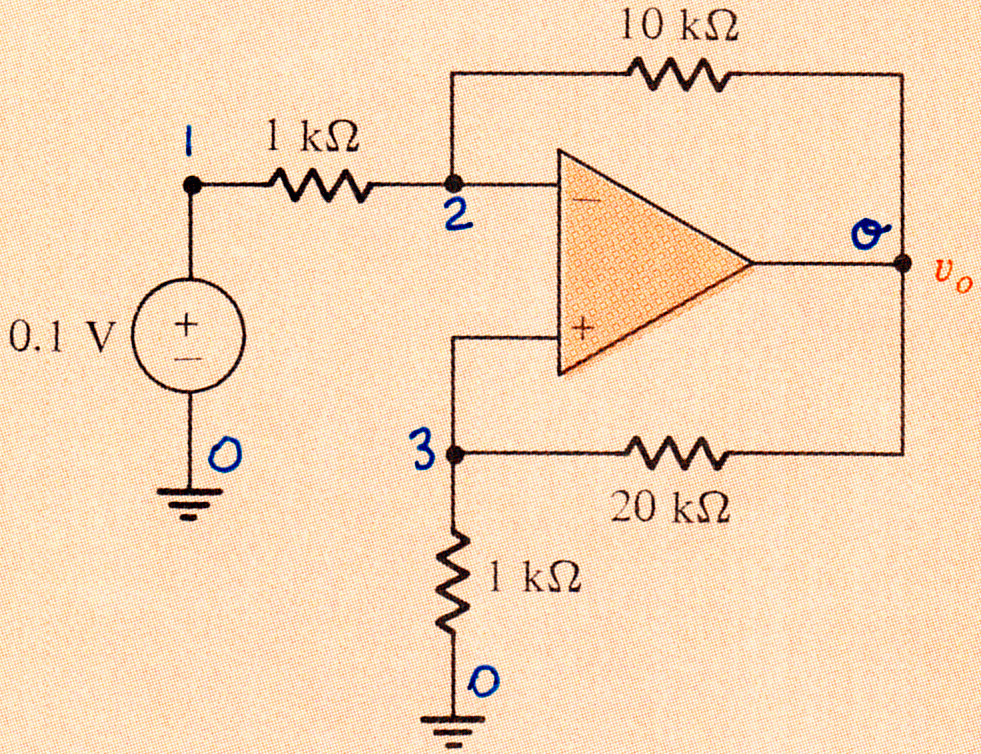
For the op-amp circuit shown, find vo and the power absorbed by the op amp.

My solution below:

s\dc("e,1,0,.1:r12,1,2,1'k:r2o,2,o,10'k:r30,3,0,1'k:r3o,3,o,20'k:o,3,2,o")

We ask for the values of the variables:

{vo,po}

The answers are {–2.1,–.00063}, which are correct. The voltage in node o is -2.1V, and the op amp is absorbing -.63 mW, which is to say it is delivering .63 mW of power to the circuit.

Instructive Op Amp examples

We have prepared a series of solved problems of circuits that include operational amplifiers. Practicing these problems will help you assimilate better what you have learned so far, before moving to the next lesson. You can download them in a PDF by clicking here.

How to describe a capacitor

For example, an ideal resistor called ca, connected between two nodes called 1 and 2, with a capacitance of 3F, and an initial condition of 0.1V, would be described in Symbulator as follows: ca,1,2,3,0.1

Values can use SI prefixes

The values of the capacitance and the initial condition of the capacitor can use prefixes of the International System (SI).

What answers do you get

For each capacitor, a transient analysis in Symbulator will provide two answers in the calculator’s memory:

• The voltage drop in the capacitor, that is to say, the voltage in the first node declared minus the voltage in the second node declared, is stored in a variable called v plus the name of the capacitor. This value is in volts.
• The current through the capacitor, flowing from the first node towards the second, is stored in a variable called i and the name of the capacitor. This value is in amperes.

Note on capacitors in DC

In a DC simulation, the current through a capacitor is defined as 0. It basically becomes an open circuit.

How to describe an inductor

For example, an ideal inductor called l1, connected between two nodes called 1 and 2, with a capacitance of 0.1H, and an initial condition of 0.2A, would be described in Symbulator as follows: l1,1,2,0.1,0.2

Values can use SI prefixes

The values of the inductance and the initial condition of the inductor can use prefixes of the International System (SI).

What answers do you get

For each inductor, a transient analysis in Symbulator will provide two answers in the calculator’s memory:

• The voltage drop in the inductor, that is to say, the voltage in the first node declared minus the voltage in the second node declared, is stored in a variable called v plus the name of the inductor. This value is in volts.
• The current through the inductor, flowing from the first node towards the second, is stored in a variable called i and the name of the inductor. This value is in amperes.

Note on inductors in DC

In a DC simulation, the voltage drop in a capacitor is defined as 0. It basically becomes a short circuit.

Running a transient analysis

You will learn the subtleties of running transient simulations in Symbulator through a series of examples presented below. For now, suffice it to say that to run a transient simulation in Symbulator, we use an access program called s\tr, which takes one argument: the circuit description in string form. Below you will find plenty of examples of TR simulations, showing you how to describe sources that are step, impulse and function of time, as well as sources that are constant, both numeric and symbolic.

For transient simulations, Symbulator uses a software for Laplace Functions made by Lars Frederiksen. Make sure you have it properly installed!

Ok, let’s get right into it, with a first example.

Solution. For t ≤ 0s, since the current source is inactive, there is nothing going on. Without doing a simulation, we know the voltage v is 0 volts.

For 0s < t ≤ 2s, the source is active. By inspection of the graph (b), we learn that for this interval the value of the source is t. That is to say, the current in amperes is the same as the time in seconds. We describe the circuit and run the transient analysis simulation using the command shown below:

s\tr("j,0,1,t:c,1,0,2,0")

Here, s\tr is the transient analysis gate and the circuit to be simulated is provided between the quotes. The description of the source has four terms: name (starting with j), first node, second node, and value. In this case the value is t. The description of the capacitor has five terms: name (starting with c), first node, second node, value in F, and the capacitor's initial condition in volts. In this case, the initial condition of the capacitor is 0 volts.

Once the simulation is complete, ask for the value of the voltage: vc. We get this value, which is correct:

t^2/4

For 2s < t, the voltage is equal to whatever value it had at time 2s:

vc|t=2

We get a value of 1 volt, which is correct.

Let's now learn more about how to describe source values, and how to think about intervals.

Describing source values

For the purpose of a transient analysis, Symbulator accepts many types of source values. The only thing you must do is describe these values properly. Below are examples on how to describe four different types of source values.

Step values: symbolic

A source with an unknown step value starting in t=0 is described using a variable and the step function u(t). For example, a voltage source e1, connected between nodes 1 and 0, with a value of V volts starting in time = 0 seconds, would be described as follows:

e1,1,0,V*u(t)

Step values: numerical

A step source with a known numerical value can also be described as above:

e1,1,0,12*u(t)

However, to save some typing, when your value is numerical, you can skip the u(t). Symbulator will assume it is a numerical step value you are passing.

e1,1,0,12

The results you get are the same. So, if you know the numerical value, you can save yourself some typing by skipping the u(t) in the value description.

Impulse values

A source with an impulse value in time t=0 is described using its value, be it symbolic or numerical, and the step function δ(t). For example, a current source j1, connected between nodes 0 and 1, with an impulse value of i amperes in time = 0 seconds, would be described as follows:

j1,0,1,i*δ(t)

Values as functions of time

A source with a value that is a function of time, such as a ramp value, or a sinusoidal or exponential value, can be described by writing the value as an expression in terms of variable t. An example is found in the problem above.

j,0,1,t

Values as function of t will activate the Impala mode, in order to save time.

Dependent values

Sources with dependent values are described as we have seen before, e.g.,

j,0,1,3*vr1

A word on intervals

For transient analyses in Symbulator, every time a switch opens or closes marks the end of a time interval and the beginning of another time interval. A simulation can only be done for one time interval. When we run a TR simulation and get answers in terms of t, this variable t must be understood as the time elapsed since the start of that interval in particular. This is a distinction without a difference as long as the interval we simulate with TR starts at t=0, which is most often the case. However, sometimes problems have switch changes in times other than t=0. Some examples are given in the solved problems, i.e. Bo2's Example 5.6, where a switch closes at t=1 second, and Bo2's Drill Exercise 5.6, where a switch closes at t=2 second. In these cases, it is important to remember that Symbulator's answers for a TR simulation are given in terms of t, where t means the time elapsed since the beginning of that interval.

Two useful tools

The only tool

Unless you indicate otherwise, a Symbulator simulation will give you a whole array of answers: voltages in all nodes, and voltage drops, currents and power consumed in all elements, etc. When the circuit you are solving has complicated symbolic expressions, storing all these answers in the memory requires time. In case you don't want all the answers, but only a chosen few, you may save some time by using the s\only tool to tell Symbulator - before the simulation - which answers you want to save. Find it in Symbulator's custom menu. The argument of s\only is either an empty variable or a string with a variable or a list of variables separated by comas, as shown below. All of these are valid:

s\only(ir1)

s\only("ir1")

s\only("ir1,va,vr2")

The s\only tool is valuable in TR analysis, because you can save time by not having Symbulator find the inverse Laplace of answers that are not needed. We show you how to use the s\only tool using a variation of a familiar example, Bo2's Drill Exercise 5.11, in the solved problems.

The plot tool

Very often we are asked to plot functions of time. The calculator has extensive plotting capabilities, but just to save you some time, Symbulator includes a handy s\plot tool that allows you to plot functions of time.

s\plot()

In the solved problems, we build upon Bo2's Example 6.1 to show you how to use it.

Instructive solved examples

We have prepared a series of solved problems of transient analysis in circuits using capacitors and inductors. Practicing these problems will help you assimilate better what you have learned so far, before moving to the next lesson. You can download them in a PDF by clicking here.

AC analysis in Symbulator

The main thing you need to know about Symbulator is that, when working on the AC mode, it understands phasors, namely complex numbers. You can analyze alternating current (AC) circuits in Symbulator by means of phasors. Symbulator uses phasors in the input, analysis and output of AC circuits.

Symbulator does not understand sinusoids. You should not feed Symbulator any sinusoids, or expect any sinusoid answers from it. Any conversion to and from sinusoids has to be done by you.

The ac program

Symbulator has a program dedicated to analyzing AC circuits. It is called s\ac. As opposed to the s\dc and s\tr programs, which only take the circuit description as their input, the s\ac program takes two inputs:

• The first is the circuit description, in a string, just as before.
• The second is the frequency of the circuit in radians per second.

The AC mode

Besides the s\ac program itself, you can use other Symbulator tool and programs, such as s\er, s\th and s\ex in their AC mode. You do this by selecting AC from the options, when asked by these programs what type of analysis you want to conduct. In this lesson, we will see examples of all of these.

Describing elements for AC

When describing a circuit for AC analysis, be it for the s\ac program or for the AC mode in other programs, you have to describe the value of elements in the correct way for this type of analysis. Valueless elements, like the short circuit and the op amp, are described the same way. Here's how to describe elements with values:

• Current sources j and voltage sources e accept complex values for AC analysis. You can declare their value in rectangular form, e.g., 10-3𝐢, or angular form, e.g., (100∠120°).
• The second is the frequency of the circuit in radians per second.
• The element r, when passed to a DC analysis, no longer represents just a resistor: it now represents an impedance. (If you are wondering why we didn't use the letter z, wait until we get to two-ports). In AC analysis, the element r accepts complex numbers as its value, such as 10-3𝐢 (where 𝐢 is the complex operator). We use r to describe resistors (by giving real values) and conductances (real values but inverted), but also to describe impedances (by giving complex values) and admittance (by giving the inverse of their complex value).
• The elements c and l are used to describe capacitors and inductors, respectively, only when their values are given to us by the problem in faradays and henrys, respectively. For AC analysis, their description no longer requires the fifth component of the initial condition, since alternating current analysis focuses on the steady state after transient effects are long gone. So, we only use the name, the two nodes, and the value of the element in faradays and henrys.

Values can use SI prefixes

The values of all of these elements can use prefixes of the International System (SI).

What answers do you get

When you run an analysis in s\ac, you get the same answers you did before in DC, except that now they are phasors. The one difference is that now, besides real power consumed, you also get the complex power consumed in these elements. We will discuss this in the next lesson.

Solved numerical examples

With values in F and H

Find v(t) and i(t).

Since this is the first AC problem we will solve, I will explain every step, including manual ones, in full detail.

Step 1: Sinusoids to phasors. We have to express the value of the source in terms Symbulator can understand. So we convert it from a sinusoid to a phasor: 10∠0°. We can pass this to Symbulator as (10∠0°) or, since it the angle is zero, simply as 10.

Step 2: Note the frequency. The circuit has a capacitor with a value given in faradays. Because of this, we know that Symbulator will ask us the frequency. The frequency is given by the problem as 4 rad/s. Symbulator will use it to convert that value from faradays to a phasor in ohms.

Step 3: Describe the circuit. We will now describe the circuit. This is my description:

"e,1,0,10:r1,1,2,5:c,2,0,.1"→cir

Notice that, in our circuit description, the order we give to the nodes of the resistor and the capacitor is chosen to be convenient for the answers we will ask. Now we pass this circuit description, and the frequency, to the ac program.

s\ac(cir,4)

Once Symbulator is done, you should take a look at the answers it stored in the current folder. There you will see:

• the usual voltages in the nodes, voltage drops in the elements, and currents through the elements, in variables that should be familiar by now.
• the average power consumed in the source and the resistor, stored in variables ape and apr. None is given for the capacitor, since capacitors and inductors do not consume real power.
• the complex power consumed in all elements, stored in variables sc, se and sr1.
• the equivalent impedance of the rest of the circuit, as seen by the source e, in a variable called ze.

The s\aa tool

To get the answers we need for this problem in particular, we ask for ir1 and vc. It is likely that the calculator will give you the answers in rectangular form, with a real part and an imaginary part. If we want to see them as an amplitude and angle, we can use Symbulator's aa tool, as follows:

s\aa(ir1)

This gives us 1.789∠26.57°, which is correct. You manually convert this to a sinusoid, by putting it back in the same terms that the input was given: 1.789 cos(4t+26.57°) A

s\aa(vc)

This gives us 4.472∠-63.43°, which is correct. You manually convert to sinusoid form: 4.472 cos(4t-63.43°) V

Future solved problems will not include this level of detail in the solution, only the circuit description and the commands we give Symbulator and the calculator.

Determine v(t) and i(t).

This is my description of the circuit:

"e,1,0,(20∠30°):r1,1,2,4:l,2,0,.2"→cir

We pass the circuit description and the frequency to ac:

s\ac(cir,10)

We ask for s\aa(ir1) and get 4.472∠3.43°, which is correct. We ask for s\aa(vl) and get 8.944∠93.43°, which is correct.

Find the input impedance of the circuit. Assume that the circuit operates at ω = 50 rad/s.

Since this is a passive circuit, to reduce it we will use the s\er tool. This is my description of the circuit:

"ca,1,2,2'm:r1,2,3,3:cb,3,0,10'm:l1,2,4,.2:r2,4,0,8"→cir

We pass the circuit description to the er tool, along with the names of the two nodes:

s\er(cir,1,0)

When asked what type of analysis, choose AC. Since there are capacitors in faradays and an inductor in henrys, Symbulator will ask you for the frequency, so it can convert them to impedances. When asked, enter 50.

Once the program is done, ask for the value of the equivalent impedance:

zeq

You get 3.22-𝐢11.07 Ω, which is correct.

(By the way, in case you were tempted to use the s\pr tool to reduce this circuit, instead of using a simulation, remember that the s\pr tool only reduces resistors and impedances. You would need to convert the capacitors and the inductor to impedances in ohms before you do that.)

Find the steady-state current i in the circuit when vs(t)=50 cos 200t V.

Here's my description:

"e,1,0,50:r1,1,2,10:c,2,3,5'm:l,3,0,20'm"→cir

I give it and the frequency to ac:

s\ac(cir,200)

We ask for s\aa(ir1) and get 4.789∠-16.7°, which is correct.

With values in Ω only

When the values of all the capacitors and inductors in the circuit are given in imaginary Ω, they must be entered in the circuit description as impedances, r. In these cases, Symbulator will not need a frequency.

Determine the admittance Y for the circuit.

Since the values are in Ω, these are all impedances. This is a passive circuit, so we could use the s\er tool. However, the structure of this circuit is so simple that we can reduce it using the s\pr tool. The problem asks for the equivalent admittance, so our answer will be the inverse of the equivalent impedance:

1/(s\pr({4,𝐢8,-𝐢10}))

Evaluating approximately, we get 0.25-0.025𝐢 S, which is correct.

For the circuit shown, find the equivalent impedance, and use that to find current I. Let ω = 10 rad/s.

Notice that the question gives us a frequency, but it is entirely superfluous. We do not need it and will not use it.

Notice also that, since we do not need anything else other than the current, it would be faster to solve this without a simulation.

First, we easily find the Z_EQ like this:

4+𝐢20+s\pr({16,-𝐢14+𝐢25})→zeq

Evaluating approximately, we get 9.135+𝐢27.469 Ω. Now we find the current by dividing the source's voltage by zeq:

s\aa(12/zeq)

We get 414.5∠-71.6° mA, which is correct.

We could also have run a simulation, reducing the impedances on the fly using the shorthand for the s\pr tool, as follows:

"e,1,0,12:r1,1,0,4+𝐢20+[16,-𝐢14+𝐢25]"→cir

No frequency is required to solve this circuit, but the s\ac program requires two inputs, so you can just leave ω or put 1 or whatever you want. Makes no difference what frequency you put.

s\ac(cir,ω)

Now ask for the equivalent impedance as seen by the source approx(ze) and for the current s\aa(ir1), and get the same answers.

Determine the equivalent impedance for the circuit.

This is my circuit description:

"r10,1,0,𝐢6:r20,2,0,𝐢8:r30,3,0,𝐢8:r40,4,0,𝐢12:r12,1,2,2:r23,2,3,-𝐢6:r34,3,4,4:r14,1,4,-𝐢4"→cir

Let's use the s\er tool.

s\er(cir,1,0)

Evaluating zeq approximately, we get 0.3794+𝐢1.4598 Ω.

Find ix in the circuit.

Describe the circuit:

"e1,1,0,20:r1,1,2,10:cx,2,0,.1:l1,2,3,1:j1,0,3,2icx:l2,3,0,.5"→cir

Run the simulation:

s\ac(cir,4)

Ask for the answer, in polar form:

s\aa(icx)

We get 7.59∠108.4°, which is correct.

Find v1 and v2 in the circuit.

Describe the circuit:

"j,0,1,10:rx,1,0,2:c,1,2,.2:l,2,0,2:r1,2,3,4:e,3,0,3vrx"→cir

Run the simulation:

s\ac(cir,2)

Ask for the answers, in polar form: s\aa(v1) and s\aa(v2)

We get 11.33∠60.02° and 33.02∠57.13°, which are correct.

Obtain vo and io in the circuit.

The book wants the answers in terms of cosine, not sine, so we use the source's value as 8 cos(1000t-40°). As a phasor, that is (8.∠–40°).

We describe the circuit:

"e1,1,0,(8.∠–40°):r1,1,2,4.'k:co,2,0,2.'µ:l1,2,3,50.'m:j1,0,3,.5ico:ro,3,0,2.'k"→cir

Notice I used decimal points after the values, to make them approximate. Run the simulation:

s\ac(cir,1000.)

Ask for the answers, in polar form: s\aa(vro) and s\aa(ico)

We get 1.55∠-95.18° V and 3.26∠-3.74° mA, which are correct.

Find V1 and V2 in the circuit.

Describe the circuit:

"j1,0,1,3.:r1,1,0,1.:rx,1,0,-𝐢1.:r3,1,2,-𝐢2:j2,1,2,.2vrx:r4,1,2,2.+𝐢2.:r5,2,0,-𝐢1.:r6,2,3,2.+𝐢2.:e1,3,0,(18.∠30°)"→cir

Notice I used decimal points after the values, to make them approximate. Run the simulation:

s\ac(cir,ω)

Ask for the answers, in polar form: s\aa(v1) and s\aa(v2)

We get 2.708∠-56.73° V and 6.914∠-80.70° mA, which are correct.

Solved numerical from symbolic examples

Calculate the value of C so that the net impedance is purely resistive at 2kHz.

The answer given by the book is 25µF. But I think this is one of those (unfortunately common) instances when there is a mistake in the book. I believe the book meant to ask "at 2k rad/s", because in that's the frequency when the answer they give, 25µF, is the right answer. Let me tell you how I solved this problem and I will let you be the judge.

Here is my circuit description:

"c,1,0,c:r1,1,2,10:l,2,0,5'm"→cir

Let's use s\er to find zeq:

s\er(cir,1,0)

When asked, specify AC. Then we are asked for the frequency. Enter the one given to us by the problem, namely 2000Hz. Symbulator asks for the frequency in rad/s, so we need to convert 2000Hz to rad/s. I do this right there, by entering 2π2E3 as the frequency. I could also have entered 12566.37, which is the equivalent value of the frequency in rad/s.

Please notice two things. First, notice that I did not use an SI prefix. The shorthand for SI prefixes only works in the circuit description string. Second, notice that I used 2E3 instead of 2000 because I wanted to have an approximate value as opposed to an exact value. The reason is that, when I tried simulating using only exact values in the input, Symbulator (well, the cSolve function working behind the scenes) was taking too long to solve the problem.

Once the simulation finishes, I ask the calculator to find the answer to our question, by solving for the value of c that makes the imaginary part of zeq equal to zero:

solve(imag(zeq)=0,c)

Initially I used cSolve here, which also works, but my friend Qifan Wang - who verified my answers to this problem - pointed, correctly, that it is not necessary to use cSolve here. Actually, using solve produces a cleaner answer because, by focusing on the imaginary part of the equation, all the references to the 𝐢 operator are gone. For practical purposes, we are solving an equation with real terms only, even though we know those terms come from the imaginary plane.

The answer is c= 0.000001235, or 1.235µF. This is not the answer the book gives.

Let's now repeat the process, using what I suspect is the frequency they meant to ask about: 2000 rad/s. I also want to show you something cool. Now that we know the answer is in the range of µF, we can declare the value of the capacitor as c'µ, so that the value of c we get will be in that scale. (If this trick confuses you, do not worry and just declare it as c.)

Here is my circuit description, using the cute c'µ trick:

"c,1,0,c'µ:r1,1,2,10:l,2,0,5'm"→cir

We use s\er to find zeq:

s\er(cir,1,0)

We specify AC and give 2000 as the frequency. When the simulation finishes, ask the calculator:

solve(imag(zeq)=0,c)

The answer is c=25, that is to say 25µF.

This is the right answer in the book. So they asked the wrong question. That is, they asked the question using the wrong frequency unit. If you liked this problem, here's another one just like it.

What is the required value of C such that the net impedance is purely resistive at 10MHz.

Same problem, different circuit. I suspect the value of the capacitor is going to be in pico or nano faradays, so I decided to define the value of the capacitor as c'p, to get the value of c in pF. (If this confuses you, just define it as c and you will get the value of c in F.)

Here is my circuit description:

"c,1,2,c'p:r1,2,0,300.:l,2,0,20'µ"→cir:s\er(cir,1,0):solve(imag(zeq)=0,c)

When asked, specify AC and enter 2π1E7 as the frequency (which is the equivalent value of 10MHz in rad/s. You get one answer: c=234.88, that is to say 235pF. This is the right answer in the book.

Solved symbolic examples

Find the input impedance Zi.

Describe the circuit, giving symbolic values to the elements as given in the circuit schematic:

"o1,1,i,i:r1,i,2,r1:r2,2,o,r2:o2,0,2,o:c,1,o,c"→cir

We use er to find zeq:

s\er(cir,1,0)

When asked, specify AC and give ω as the frequency. We also pass the circuit a symbolic frequency, not because it's not needed, but because we want the analysis to use a symbolic frequency as input.

We ask for the answer: zeq and get a symbolic expression: -r1/(c*(r1+r2)*ω)*𝐢. It looks somewhat different to the answer given in the book, because they rearranged the terms, but they are the same thing.

Find Vo/Vs.

Describe the circuit:

"e,1,0,vs:c,1,2,c:r1,2,o,r:o,0,2,o"→cir

Run the simulation, with a symbolic frequency:

s\ac(cir,ω)

We ask for the answer: vo/vs and get -c*ω*r*𝐢, which is correct.

Know Symbulator's limits

Symbulator is a calculator program. It runs on a limited hardware, supported by a limited CAS. It can solve most of the problems you will find in the textbooks used in Circuits I and II courses. It particularly shines when solving symbolic problems.

However, as you move to larger and more complex problems, Symbulator will struggle to solve them. In a sense, this is not a problem. First, because it makes no sense to solve large circuits symbolically: the resulting expressions are beyond our understanding. Second, because there are already many established tools to solve such large circuits numerically.

What matters here is that you know the limits of Symbulator, so that they don't take you by surprise in an exam. Think of Symbulator as a wonderful "Swiss knife" of circuit simulator: no matter how good it is, it is still a pocket knife. You would not try to chop a tree down with it. For that you would use a chainsaw or an axe. SPICE and its children (LTspice, PSpice, MultiSim, etc.) are the chainsaws of circuit simulation. They won't run on your calculator, nor give you symbolic answers, but when you need to chop a tree down, they are the way to go.

We will now see an example that takes Symbulator and its platform to the limit of what they can solve symbolically.

Compute the closed-loop gain Vo/Vs for the op amp circuit.

Describe the circuit:

"e,1,0,vs:r1,1,2,r1:ca,2,0,ca:r3,0,3,r3:o,2,3,o:cb,3,o,cb:r2,3,o,r2"→cir

Run the simulation, with a symbolic frequency:

s\ac(cir,ω)

We ask for the answer: vo/vs and get a huge expression, shown here:

Looks different from the answer in the book, but I evaluated it and it is the same as the answer given in the book, but arranged differently.

Average Power

Determine the load impedance ZL that maximises the average power drawn from the circuit. What is the maximum average power?

Symbulator's th tool help us find all the answers we need. Here is the circuit description I will give it:

"e,1,0,10:r1,1,2,4:r2,2,0,8-6𝐢:r3,2,3,5𝐢"→cir

Notice this circuit description does not include the load, because it is not needed in the input to the th tool.

s\th(cir,3,0)

When asked a type of analysis, specify AC. Then you will be asked if a load problem is next. You don't have to answer Yes, but I invite you to do so, because I want to show you something cool with what you get from that.

When the tool is done running, check what variables were stored in the memory.

The er tool saves for you the equivalent impedance of this circuit, in a variable called zeq. The load that will deliver the maximum power is the conjugate of the zeq. You can find it by asking: conj(zeq), which evaluates approximately to 2.933+𝐢4.467.

The er tool saves for you the average maximum power delivered by the circuit, in a variable called apmax, which evaluates approximately to 2.3674 W.

Now, here's the cool part: When you answer Yes to the load question, Symbulator saves expressions for the current through, voltage drop in, average power and complex power in a load connected to the equivalent circuit, as a function of the complex value of that load (the variable load_, where the underscore tells the calculator to treat this variable as complex). This means that you can verify that this is the maximum power delivered, by evaluating the value of the average power in the load when the load is equal to the conjugate of the equivalent impedance.

aprl|load_=conj(zeq) evaluates to the same answer.

RMS and PF

In the previous lesson, we mentioned that after an AC simulation, besides real power consumed, you also get the complex power consumed in these elements. This complex power is stored in a variable called s and the name of the element. The way you should interpret these values will depend on the setting of a flag called the RMS flag.

The userms flag

You will learn in your circuits course or textbook that phasor analysis can be conducted using something called RMS values. There are certain advantages to this, and you will have to solve AC circuits both in normal values (also called magnitude values) and in RMS values. Working in RMS values basically means that all the currents and voltages in the analysis are considered to be RMS. That's it.

There is a flag in Symbulator that tells the program whether you want to conduct your analysis in normal values or in RMS values. That flag is stored in a variable called userms, and it can have the value of true or false. By default, this flag has a value of false.

When the flag has this false value, AC analysis is conducted assuming normal values are used. Symbulator will assume that all the currents and voltages you give it are in normal values, e.g., magnitude values. It will give you all the current and voltage answers in normal values as well. And after an s\ac analysis, you will get the average real power consumed in r, e, j and o elements stored in a variable called ap and the name of the element.

On the other hand, when the RMS flag has a value of true, AC analysis is conducted assuming RMS values are used. Symbulator will assume that all the current and values that you feed it are in RMS values. It will give you all the current and voltage answers in RMS values as well. And after an s\ac analysis, you will get the average real power consumed in r, e, j and o elements stored in a variable called p and the name of the element.

Determine the power factor of the entire circuit as seen by the source. Calculate the average power delivered by the source.

The source value in this problem is given in RMS values. So that Symbulator knows to interpret the value you gives for it as being RMS, we must set the userms flag to true:

true→userms

We can describe the circuit in full, like this:

"e,1,0,30.:r1,1,2,6.:r2,2,0,–𝐢2.:r3,2,0,4."→cir

Or, if you want to simplify the impedances, like this:

"e,1,0,30.:r1,1,0,6.+[–𝐢2.,4.]"→cir

Notice we are using decimal points in the values. Run the simulation:

s\ac(cir,ω)

The average power consumed by the source is stored in a variable pe. To get the average power delivered, we ask for the negative of it: –pe, which gives us 125.4 W.

The s\pf tool

To find the power factor of an element answer, we can use the s\pf tool. We can use this tool in two ways.

With a complex expression as input

One way to use the pf tool is by giving as its input a complex expression, i.e., one with real and imaginary parts. This complex expression can contain symbolic and/or numerical values, be them exact or approximate. It can be a complex number, in rectangular or angular form. The input can also be a variable stored in memory that contains such a complex expression, such as the variable that stores the complex power consumed or delivered in an element.

For example, to get the power factor of the source in the circuit we just simulated, based on their complex power, se, we ask for:

s\pf(se)

The pf tool takes this complex value, and calculates the power factor as the absolute value of the real part divided by the magnitude of the whole thing.

Now, this is not the whole picture: we need to know if this power factor is leading or lagging. The pf tool can help you with that when the answers to a circuit simulation are numerical, as we will see below.

With an element name as input

The second way to use the pf tool is by giving it as input a string with the name of a single element that was part of an s\ac simulation that just finished. The tool recognizes three elements in this second form: e, j and r:

For example, to get the power factor of the source e in the circuit we just simulated, we ask for:

s\pf("e")

We get that the power factor is 0.97342, and we also get that it is leading.

So, in a nutshell: If you give pf as input a complex number or expression, or a variable that contains one, you will get a number or expression for the power factor, but no indication of whether it is leading or lagging. And if you give pf as input the name of an element in a string, right after an s\ac simulation, then we will get as an answer, in a string, the value and a verbal description of lagging or leading. This second will only work if the expression can be evaluated numerically (e.g. no symbols in it).

Let's see another example, just like this one, so you can practice.

Calculate the power factor of the entire circuit as seen by the source. What is the average power supplied by the source?

My solution:

true→userms:"e,1,0,165.:r1,1,0,10.+[𝐢4.,8.-𝐢6.]"→cir:s\ac(cir,ω)

–pegives us 2007.1 W.

s\pf("e") gives us pf: 0.93595 leading.

If exact fails, try approximate

Fun fact: This circuit cannot be solved in Symbulator if you give it the full circuit description with exact values. If you describe it like this:

"e,1,0,165:r1,1,2,10:r2,2,0,𝐢4:r3,2,3,8:r4,3,0,-𝐢6"

...the simulation will result in a resource exhaustion error, due to the bug in cSolve in the TI-Nspire's CAS. But if you add decimal points, like this:

"e,1,0,165.:r1,1,2,10.:r2,2,0,𝐢4.:r3,2,3,8.:r4,3,0,-𝐢6."

...the simulation will run just fine.

A power transmission system is modeled as shown. If Vs=240 rms, find the average power absorbed by the load.

Easy peasy:

true→userms:"evs,1,0,240.:rl1,1,2,.1+𝐢:rl,2,3,100+𝐢:rl2,3,0,.1+𝐢"→cir:s\ac(cir,ω):prl

We get 573.2 W.

Complex Power

The figure shows a load being fed by a voltage source through a transmission line. The impedance of the line is represented by the (4+j2) Ω impedance and a return path. Find the real power and reactive power delivered by the source, and absorbed by the line and load.

The value of this circuit's source is given in RMS, so:

true→userms

Since the problem asks for answers regarding the line and the load, we should have separate impedances, one for the line and one for the load.

"e1,1,0,220.:r1,1,2,4.+2.𝐢:r2,2,0,15.-10.𝐢"→cir:s\ac(cir,ω)

The complex power absorbed in the source, line and load are stored in these variables:

{-se1,sr1,sr2}

We get these answers, which are correct:

{2163.8-911.1*𝐢,455.5+227.8*𝐢,1708.2-1138.8*𝐢}

Consider the power system shown. Calculate: (a) the total complex power, (b) the power factor, and (c) the parallel capacitance necessary to establish a unity power factor.

The values are in RMS, so:

true→userms

This is my circuit description:

"e,1,0,240:r1,1,0,80-𝐢50:r2,1,0,120+𝐢70:r3,1,0,60+𝐢0"→cir

We do not need to bother with the frequency for the first two questions.

s\ac(cir,ω)

To answer (a), we get the complex power delivered by the source as follows:

–se, which gives us 1835.9-114.7*𝐢 VAR.

To answer (b), we get the power factor in the source. Since we are interested in the direction (e.g. lagging or leading), and the answers of the simulation are numerical, we can give s\pf the name of the source "e" as input, as follows:

s\pf("e"), which gives us that pf: .99805 leading.

To answer (c), we need to run a new simulation, with a capacitor with a symbolic value, and then get an expression for the power factor as a function of that capacitor's value, which we will use to find how much that value will be when the power factor is 1. This is how we do that:

First, we add a capacitor to the circuit, in parallel, with a symbolic value (let's say x):

"e,1,0,240:r1,1,0,80-𝐢50:r2,1,0,120+𝐢70:r3,1,0,60+𝐢0:c,1,0,x"→cir

Since now we have a capacitor, with a value in faradays, we do need to give the simulation a frequency. The problem states its 50Hz, which is (2π)(50) in rad/s.

s\ac(cir,2π50.)

Now, if you ask the calculator for s\pf(se), you will see that it produces an expression for the power factor that is a function of the value x. Which means we can solve to find what value of x makes it equal to 1.

solve(s\pf(se)=1.,x)

This returns a value of -6.3 μF. No positive value satisfies this equation, only this negative value. Maybe that's why the book does not give a numerical answer for (c). I decided to try with an inductor instead.

"e,1,0,240:r1,1,0,80-𝐢50:r2,1,0,120+𝐢70:r3,1,0,60+𝐢0:l,1,0,x"→cir

s\ac(cir,2π50.)

solve(s\pf(se)=1.,x)

This returns a value of 1.5987 H. This value is positive, so this is our answer.

We can verify that this is the correct answer by running a simulation with that result as the numerical value of the inductor:

"e,1,0,240:r1,1,0,80-𝐢50:r2,1,0,120+𝐢70:r3,1,0,60+𝐢0:l,1,0,1.5987"→cir:s\ac(cir,2π50.)

If you then ask for s\pf(se) or s\pf("e"), you see that the resulting pf of the circuit as seen by the source is basically 1. This verifies that the correct answer is adding an inductor of 1.6H in parallel.

About solving three-phase circuits

Three-phase circuits can be tricky to solve in Symbulator, for several reasons. For example, it is not always clear which node should be used as ground node. There are three times as many nodes as there would be for an equivalent single-phase circuit. And, in the case of sources in a delta array, there are some mathematical issues, where we have more unknowns than equations.

Symbulator does great job of solving the simple three-phase circuits that you may encounter in a basic Circuits I / II textbook. Here we will see some examples, and one or two tricks, to solve them. Having said, that, Symbulator would not be my tool of choice for solving anything larger than such basic circuits. As circuits grow larger, the number of nodes quickly grows beyond what the calculator can solve.

Wye-Wye

Balanced Wye-Wye System

Calculate the line currents in the three-wire Y-Y system. Determine the total average power, reactive power, and complex power absorbed at the source and at the load. (Note: Assume that the values given for the source are RMS.)

Although not specified in the textbook, to get the answers they give we need to assume that the values are RMS, so I added that note above. We need to set the RMS flag as true:

true→userms

One must describe the circuit carefully in the case of three-phase circuits, because it's very easy to make a mistake. Below is how I describe this circuit:

"ea0,ag,0,(110.∠0°):eb0,bg,0,(110.∠–120°):ec0,cg,0,(110.∠120°):rat,ag,ad,5.-𝐢2.:rbt,bg,bd,5.-𝐢2.:rct,cg,cd,5.-𝐢2.:ra0,ad,0,10.+8.𝐢:rc0,cd,0,10.+8.𝐢:rb0,bd,0,10.+8.𝐢"→cir:s\ac(cir,ω)

Some observations about my description:

• Notice that I have specified the node at the center of both Y's as node 0. This is something you can do only in the case of balanced Y-Y systems, but not for other configurations and not for unbalanced systems.
• Since the calculator does not differentiate between lower and upper case variables, names called a and A would be considered the same node. Instead, we use the names ag and ad for these nodes, where the g reminds us a node is on the generation side and the d reminds us a node is on the demand side.

Once the simulation is completed, we ask for the currents on the transmission lines, as follows:

{s\aa(irat),s\aa(irbt),s\aa(irct)}

We get the following answers, which are correct:

{"6.809ᴇ0∠-21.8°","6.809ᴇ0∠-141.8°","6.809ᴇ0∠98.2°"}

The complex power at the source is given by:

sea0+seb0+sec0

The complex power is the whole answer:

–2086.2-834.5*𝐢 VA

The real part of that answer is the average power absorbed by the source. Since it is negative, we know the source is delivering an average power of 2086 W. The imaginary part of the answer is the reactive power: 834 VAR.

The complex power at the source is given by:

sra0+srb0+src0

The complex power is the whole answer:

1390.8+1112.6*𝐢 VA

The load is consuming an average power of 1391 W and a reactive power of 1113 VAR.

That concludes the solution to this problem. Before we move to the next, I want you to try simulating this circuit using a different node, other than 0, as the centre of the Y array of the load. I called that node d0, to remind me it's the centre for the demand side. Like this:

"ea0,ag,0,(110.∠0°):eb0,bg,0,(110.∠–120°):ec0,cg,0,(110.∠120°):rat,ag,ad,5.-𝐢2.:rbt,bg,bd,5.-𝐢2.:rct,cg,cd,5.-𝐢2.:ra0,ad,d0,10.+8.𝐢:rc0,cd,d0,10.+8.𝐢:rb0,bd,d0,10.+8.𝐢"→cir:s\ac(cir,ω)

If you evaluate the voltage in this node, like this:

vd0

You will see that the voltage is 0 V, because the system is balanced. That's why we were able to use 0 as that node. When we solve an unbalanced system, we cannot use 0 in both nodes.

Also, calculate the complex power at the source and at the load. (Assume the source voltage is given as RMS.)

We set the RMS flag as true, because - although the textbook doesn't mention it - you will only get the right answers if you assume the values here are RMS.

true→userms

Then, we describe the circuit. Notice that we have three impedances in each line: one inside the generator, one for the transmission line, and one for the load. I have given the nodes between them names that will remind me that they are in the generator, on the supply side, and on the demand side:

"ea0,ag,0,(120.∠30°):eb0,bg,0,(120.∠–90°):ec0,cg,0,(120.∠150°):rag,ag,as,.4+𝐢.3:rbg,bg,bs,.4+𝐢.3:rcg,cg,cs,.4+𝐢.3:rat,as,ad,.6+𝐢.7:rbt,bs,bd,.6+𝐢.7:rct,cs,cd,.6+𝐢.7:ra0,ad,0,24.+19.𝐢:rb0,bd,0,24.+19.𝐢:rc0,cd,0,24.+19.𝐢"→cir:s\ac(cir,ω)

Now, the question asks for the line voltages, e.g., the voltage difference between the lines. To get the answer they want, you ask for:

{s\aa(vag-vbg),s\aa(vbg-vcg),s\aa(vcg-vag)}

This will get you the answers given in the textbook:

{"207.8ᴇ0∠60.°","207.8ᴇ0∠-60.°","207.8ᴇ0∠180.°"}

Now, if you ask me, that is not really the voltage difference between the lines, because the transmission line starts after the generator. To find the voltage between lines at the start of the transmission line, we ask for:

{s\aa(vas-vbs),s\aa(vbs-vcs),s\aa(vcs-vas)}

{"204.6ᴇ0∠60.03°","204.6ᴇ0∠–59.97°","204.6ᴇ0∠–179.97°"}

And for the voltage between lines at the end of the transmission line, we ask for:

{s\aa(vad-vbd),s\aa(vbd-vcd),s\aa(vcd-vad)}

{"198.7ᴇ0∠59.71°","198.7ᴇ0∠–60.29°","198.7ᴇ0∠179.71°"}

To get the current in the lines, we ask for:

{s\aa(irat),s\aa(irbt),s\aa(irct)}

{"3.748ᴇ0∠–8.66°","3.748ᴇ0∠–128.66°","3.748ᴇ0∠111.34°"}

To get the complex power absorbed at the source, we ask for:

sea0+seb0+sec0

–1053.7-842.9*𝐢

This is what the book is going for. Notice this does not include the complex power in the internal impedances of the source, which we could include.

To get the complex power absorbed at the load, we ask for:

sra0+srb0+src0

1011.5+800.8*𝐢

That concludes this problem.

Unbalanced Wye-Wye System

For the unbalanced circuit in the figure, find (a) the line currents, (b) the total complex power absorbed by the load, and (c) the total complex power absorbed by the source.

Since the values of the source are in RMS:

true→userms

I described the circuit as follows, using the node at the centre of the generator array as my ground, and naming node at the centre of the load as n:

"ea,a,0,(120.∠0°):eb,b,0,(120.∠–120°):ecc,c,0,(120.∠120°):ra,a,n,5.𝐢:rb,b,n,10.:rcc,c,n,–10.𝐢"→cir:s\ac(cir,ω)

This gets us all the answers we need:

{s\aa(ira),s\aa(irb),s\aa(ircc),sra,srb,srcc,sea,seb,secc}

We get the following, which are correct:

{"56.78ᴇ0∠0.°","25.46ᴇ0∠135.°","42.76ᴇ0∠–155.1°",16122.*𝐢,6480.,–18282.*𝐢,–6814.,790.6-2951.*𝐢,–456.5+5111.*𝐢}

These are all correct. You can verify the conservation of complex power by verifying that:

sea+seb+secc+sra+srb+srcc

is equal to 0. and you can verify that the voltage at the centre of the unbalanced load is not zero, by asking:

vn

We get that the voltage in N is 120.-283.9*𝐢 V.

The unbalanced Y-load shown in the figure has balanced voltages of 100V in the acb sequence. Calculate the line currents and the neutral current. Take ZA=15 Ω, ZB=10+j5 Ω, ZC=6-j8 Ω.

The source values are not RMS this time, so:

false→userms

We describe the circuit, noting that this time there is a neutral line running from the centre of the load array to the centre of the source array. We describe it using a short circuit. Notice also that the angles of the sources are as per the acb sequence. This is my description:

"ea,a,0,(100.∠0°):eb,b,0,(100.∠120°):ecc,c,0,(100.∠–120°):sn,0,n:ra,a,n,15:rb,b,n,10.+𝐢5.:rcc,c,n,6.-𝐢8."→cir:s\ac(cir,ω)

To get the four currents, we ask:

{s\aa(ira),s\aa(irb),s\aa(ircc),s\aa(isn)}

And we get:

{"6.667ᴇ0∠0.°","8.944ᴇ0∠93.43°","10.000ᴇ0∠-66.87°","10.06ᴇ0∠178.47°"}

This is correct.

Wye-Delta

Balanced Wye-Delta

No reference is made to these values being RMS, so you can set the flag to false. Since they are not asking for powers, it makes no difference. We give the sources the angle values that correspond to the abc sequence.

"ea0,a,0,(100.∠10°):eb0,b,0,(100.∠–110°):ec0,c,0,(100.∠130°):rab,a,b,8.+4.𝐢:rca,c,a,8.+4.𝐢:rbc,b,c,8.+4.𝐢"→cir:s\ac(cir,ω)

We get the phase currents by asking:

{s\aa(irab),s\aa(irbc),s\aa(irca)}

{"19.36ᴇ0∠13.43°","19.36ᴇ0∠-106.57°","19.36ᴇ0∠133.43°"}

We get the line currents by asking:

{s\aa(–iea0),s\aa(–ieb0),s\aa(–iec0)}

{"33.54ᴇ0∠-16.57°","33.54ᴇ0∠-136.57°","33.54ᴇ0∠103.43°"}

That's it.

For the balanced Y-Δ circuit, find the line current IaA, the phase voltage AB, and the phase current IAC. Assume that the source frequency is 60Hz.

No reference is made to these values being RMS, so you can set the flag to false. Since they are not asking for powers, it makes no difference.

This is my description:

"ea1,na1,0,(100.∠0°):eb1,nb1,0,(100.∠–120°):ec1,nc1,0,(100.∠120°):raa,na1,na2,1:rbb,nb1,nb2,1:rcc,nc1,nc2,1:rac,na2,nc2,100.+24.*π*𝐢:rcb,nc2,nb2,100.+24.*π*𝐢:rba,nb2,na2,100.+24.*π*𝐢"→cir:s\ac(cir,ω)

We get the answers by asking:

{s\aa(iraa),s\aa(vna2-vnb2),s\aa(irac)}

{"2.35∠-36.2°","169.94∠30.8°","1.36∠-66.2°"}

That's it.

Unbalanced Wye-Delta

If you find a simple unbalanced wye-delta problem, let me know.

Delta-Delta

Balanced Delta-Delta

So far, we have had no issue selecting a ground node: the natural candidate was the centre of the Y array of sources. In the case of a Δ array, however, there is no centre node. That's one problem. It can be solved by picking one of the sides of the delta on the generator side to serve as the ground node.

Another problem is that a triangle made of sources is something that doesn't sit well with simulators. SPICE-like simulators don't like it, and Symbulator doesn't like it either. In the case of Symbulator, the problem is that the third source is not adding any new information (the first two sources already define the voltage relationships between three nodes of the delta) but it is adding a new unknown, namely the current through it. Once the redundant equation is dropped by the calculator's cSolve function, the resulting system of equations has one too many unknowns and cannot be solved.

I've discovered a trick that can be used in Symbulator to simulate sources in a delta configuration. The trick consists of using only two voltage sources. These two sources sufficiently define the voltages in the three nodes of the delta. The pro of this trick is that it allows us to simulate what effect these three voltages have on the rest of the circuit. The con is that we do not have a clear idea of what is happening inside the sources in terms of currents, because the currents we get for the two sources we are using is not the current they would have in a three source configuration.

For now, that's the best I've come up with. If you think of something else, let me know. Now, let's see some examples.

A balanced Δ-connected load having an impedance of 20-j15 Ω is connected to a Δ-connected, positive-sequence generator having Vab = 330∠0° V. Calculate the phase currents of the load and the line currents.

No reference is made to these values being RMS, so you can set the flag to false. Since they are not asking for powers, it makes no difference.

Since we want to find the current in the lines, we need to add three short circuits to serve as lines between the generator and the load.

Regarding the source, we will describe it using two sources. In this particular circuit, I select the node c to serve as ground (so it will be called 0 instead of c). And the source I will leave out of the description is the one opposite to this node. Here is my description:

"e0a,0,ag,(330.∠120°):eb0,bg,0,(330.∠–120°):sat,ag,ad:sbt,bg,bd:sct,0,cd:rab,ad,bd,20.-15.𝐢:rbc,bd,cd,20.-15.𝐢:rca,cd,ad,20.-15.𝐢"→cir:s\ac(cir,ω)

To get the currents in the lines, we ask for the currents in the shorts:

{s\aa(isat),s\aa(isbt),s\aa(isct)}

We get:

{"22.86ᴇ0∠6.87°","22.86ᴇ0∠-113.13°","22.86ᴇ0∠126.87°"}

This is correct.

Unbalanced Delta-Delta

The unbalanced Δ-load of the figure below is supplied by balanced line-to-line voltages of 440 V in the positive sequence. Find the line currents. Take Vab as a reference (for the angles).

My description:

false→userms:"e0a,0,ag,(440.∠120°):eb0,bg,0,(440.∠–120°):sla,ag,ad:slb,bg,bd:slc,0,cd:rab,ad,bd,10.-𝐢5.:rbc,bd,cd,16.:rca,cd,ad,8.+𝐢6."→cir:s\ac(cir,ω)

To get the answers, we ask:

{s\aa(isla),s\aa(islb),s\aa(islc)}

We get:

{"39.71ᴇ0∠-41.07°","64.12ᴇ0∠-139.77°","70.13ᴇ0∠74.27°"}

That's correct.

Find the line currents in the unbalanced three-phase circuit and the real power absorbed by the load.

My description:

true→userms:"e0a,0,ag,(220.∠–120°):eb0,bg,0,(220.∠120°):sla,ag,ad:slb,bg,bd:slc,0,cd:rab,ad,bd,-𝐢5.:rbc,bd,cd,𝐢10.:rca,cd,ad,10."→cir:s\ac(cir,ω)

To get the answers:

{s\aa(isla),s\aa(islb),s\aa(islc),prca+prab+prbc}

We get:

{"64.00ᴇ0∠80.1°","38.11ᴇ0∠–60.°","42.50ᴇ0∠–135.°",4840.0}

This is correct.

Consider the unbalanced Δ-Δ circuit in the figure. Use PSpice to find the generator current Iab, the line current IbB and the phase current IBC.

The first of the questions refers to a current in the generator. Now, that one we won't get from Symbulator. But the other two we will.

My description:

false→userms:"e0a,0,ag,(208.∠130°):eb0,bg,0,(208.∠–110°):rla,ag,ad,2.+𝐢5.:rlb,bg,bd,2.+𝐢5.:rlc,0,cd,2.+𝐢5.:rab,ad,bd,50.:rbc,bd,cd,𝐢30.:rca,cd,ad,–𝐢40."→cir:s\ac(cir,ω)

To get the second and third answers, we ask:

{s\aa(irlb),s\aa(irbc)}

We get:

{"9.106ᴇ0∠168.48°","5.500ᴇ0∠172.47°"}

The third answer is trickier. They are asking for the current in the source we did not use in the simulation. And even if they had asked for the current in one of the sources we did have, we would not be able to trust that current, since we only used two sources and in reality the circuit uses three.

Now, I tried something, and I think I got lucky, because I got the answer the book gives. This is what I tried:

s\aa(–(ie0a+ieb0)/3)

What I thought was: the current that I have coming out of the two souces in my simulation would, in reality, be coming out of three sources. So, if I add up those two currents together, and divide them by three, I may get an approximate of the current that would be coming out of one source. I am confident that this should be the case in a balanced circuit. But this is not a balanced circuit. Still, it's the best I had to go by. So I tried it.

"5.959ᴇ0∠-177.18°"

And it worked. That's the answer in the book.

Delta-Wye

The Δ-Y configuration is the platypus of three-phase systems. One easy way to solve them is to convert the Δ source to a Y source with the transformed values, and then solve it as a Y-Y system. That may be the wise thing to do.

However, below I will show you a way I found to solve it in Symbulator. Basically, we designate the node at the centre of the Y load to serve as ground. And, as before, we simulate the Δ source using only two sources.

Balanced Delta-Wye

Here is my circuit description:

false→userms:"eca,c,a,(210.∠120°):ebc,b,c,(210.∠–120°):ra,a,0,40.+𝐢25.:rb,b,0,40.+𝐢25.:rcc,c,0,40.+𝐢25."→cir:s\ac(cir,ω)

We get the answers by asking:

{s\aa(ira),s\aa(irb),s\aa(ircc)}

This is what we get:

{"2.570ᴇ0∠-62.01°","2.570ᴇ0∠177.99°","2.570ᴇ0∠57.99°"}

This is correct.

Unbalanced Delta-Wye

If you find a simple unbalanced delta-wye problem, let me know.

How to describe a mutual inductance

In the textbooks used in Circuits I and II, you will encounter mutual impedances described in two ways:

• You will find mutual impedances with values in jΩ, coupling two inductors with values also given in jΩ.
• You will find mutual impedances with values in H, coupling two inductors with values also given in H.

Symbulator accepts both types of description, through the same element: m.

Example #1: A mutual inductance called m1, coupling two inductors with values in H called l1 and l2, with a value of 1.1 H, would be described in Symbulator as follows: m1,l1,l2,1.5

Example #2: A mutual inductance called m1, coupling two inductors with values in jΩ called r1 and r2, with a value of 2 jΩ, would be described in Symbulator as follows: m1,r1,r2,2

Mind the sequence

A crucial element in the description of the elements coupled with a mutual inductance is the polarity or direction of this coupling. This is typically indicated, in circuit schematics, with a dot. In Symbulator, the role of that "dot" is played by the sequence in which you list the nodes in the description of these coupled elements. Imagine, for example, that the first node you declare in each of these elements is the dotted one. Keep it consistent.

Values can use SI prefixes

The value of the mutual inductance can use prefixes of the International System (SI).

What answers do you get

No answers are produced for the mutual inductance.

Instructive examples with mutual inductances

Calculate the phasor currents I₁ and I₂ in the circuit.

In my description below, I want you to notice the following:

• The bottom node on both halves of the circuit is the ground node.
• The inductors and mutual inductance have values given in jΩ. So, we declare the inductors as r elements with imaginary values.
• Notice the value of the mutual inductance element is given as an imaginary number as well, so that it is consistent.
• The 'dotted' node on both coupled elements is given first in their description. This captures the polarity and is critical.

Ok, here it goes:

false→userms:"e,1,0,12:r1,1,2,-𝐢4:r2,2,0,𝐢5:m,r2,r3,𝐢3:r3,3,0,𝐢6:r4,3,0,12"→cir:s\ac(cir,ω)

To get the answers, we ask:

{s\aa(ir2),s\aa(ir4)}

We get:

{"13.02ᴇ0∠-49.4°","2.910ᴇ0∠14.04°"}

That's correct.

Determine the voltage V_o in the circuit.

In my description, notice how I define the coupled inductor starting with the dotted node first.:

false→userms:"e,1,0,(200.∠45°):r1,1,2,4.:r2,2,0,𝐢8.:m,r2,r3,𝐢1.:r3,0,o,𝐢5.:r4,o,0,10"→cir:s\ac(cir,ω)

To get the answers, we ask:

s\aa(vo)

We get:

"20.00ᴇ0∠-134.43°"

That's correct.

Calculate the mesh currents in the circuit.

My description. Notice the sequence of the nodes, matching the dots:

false→userms:"e,1,0,100.:r1,1,2,4.-𝐢3.:r2,2,0,𝐢6.:m,r2,r3,𝐢2.:r3,3,2,𝐢8.:r4,3,0,5"→cir:s\ac(cir,ω)

To get the answers, we ask:

{s\aa(ir1),s\aa(ir4)}

We get:

{"20.30ᴇ0∠3.5°","8.693ᴇ0∠19.03°"}

That's correct.

In the circuit, calculate the input impedance and current I₁. Take Z₁=60-j100 Ω, Z₂=30+j40 Ω, and Z_L=80+j60 Ω.

My description:

false→userms:"e,1,0,(50.∠60°):r1,1,2,60.-𝐢100.:r2,2,0,𝐢20.:m,r2,r3,𝐢5.:r3,3,0,𝐢40.:r4,3,4,30.+𝐢40.:rl,4,0,80.+𝐢60."→cir:s\ac(cir,ω)

To get the answers, we ask:

{ze,s\aa(ir1)}

We get:

{60.09-80.11*𝐢,"499.3ᴇ-3∠113.13°"}

That's correct.

Use PSpice to find i₁, i₂, and i₃ in the circuit displayed.

My description:

false→userms:"e1,1,0,(60.∠–10°):e2,3,0,40.:r2,1,4,100.:r1,1,2,70.:l4,2,3,2.:l1,5,4,3.:l2,5,3,3.:l3,6,5,4.:c,6,0,270'µ:m1,l1,l2,1.:m2,l1,l3,1.5:m3,l2,l3,2."→cir:s\ac(cir,12.*π)

To get the answers, we ask:

{s\aa(–ie1),s\aa(ir1),s\aa(–ie2)}

We get:

{"417.3ᴇ-3∠-72.61°","211.4ᴇ-3∠-75.75°","237.8ᴇ-3∠115.69°"}

These are the correct answers, but they are not the answers that you will find in the book. I think there is a mistake in the book.

Here I want to tell a little story, to illustrate how simple to use Symbulator is. I solved this circuit on my first try. But my answers didn't match the book, so I contacted my friend Qifan Wang and asked him to simulate it in GnuCAP. His first couple of attempts had mistakes in the description, but when he got it right, he confirmed that his answer matched that of Symbulator. We both believe that the book is wrong. I think the book made more than one mistake, by the way. Qifan's description of this circuit for GnuCAP is available here, if you want to try it.

Find i_o in the circuit, using PSpice.

Notice in my description that I decided to put the ground in the node at the middle. It felt like a good place.

false→userms:"e,6,5,(160.∠50°):r1,6,1,20.:r2,2,3,12.:r3,0,5,10.:ro,4,5,8.:c,0,4,25'm:l1,1,0,5.:l2,0,2,4.:m,l1,l2,.4*√(5.*4.):l3,3,4,6."→cir:s\ac(cir,4)

To get the answers, we ask:

s\aa(iro)

We get:

"2.011ᴇ0∠68.51°"

That's correct.

How to describe an ideal transformer

An ideal transformer has four nodes: two nodes on one side, and two nodes on the other side. In Symbulator, it is possible to simulate transformers that have one node on each side connected to the ground node. That is to say, only one node on each side is to be connected to a non-ground node.

Example #1: An ideal transformer called t1, connected on the first side to node 1 and to ground, and connected on the second side to node 2 and to ground, with 80 turns on the first side, and 800 turns on the second side with the same polarity, would be described in Symbulator as follows: t1,1,2,80,800

Example #2: An ideal transformer called t, connected on the first side to node a and to ground, and connected on the second side to node b and to ground, with a ratio of 1 on the first side to 5 on the second side, with opposite polarities, would be described in Symbulator as follows: t,a,b,1,-5 (notice the negative sign, to indicate the inversion of polarity).

What answers do you get

For an ideal transformer, the following answers are provided:

• The voltage in the two non-ground nodes where it is connected, in volts, as usual with all the nodes mentioned in the circuit description.
• The current entering the transformer through each of the two non-ground nodes, in amperes, stored in two variables called i plus the name of the transformer and the name of each node. For example, for a transformer called ta connected to nodes 1 and 2, we will get two variables called ita1 and ita2, with the current entering the transformer at nodes 1 and 2 respectively.

Instructive examples with ideal transformers

Obtain V_Th and Z_Eqfor the part of the circuit right of the a and b nodes.

In my description below, I want you to notice that the bottom node on both halves of the circuit is the ground node. For this problem, we ignore the part of the circuit that is left of the a and b nodes. Here it goes:

"t,2,3,1,n:r2,3,4,z2:e2,4,0,vs2"→cir:s\th(cir,2,0)

When asked, specify AC. To get the answers, we ask:

{vth,zeq}

We get:

{vs2/n,z2/n^2}

That's correct.

For the ideal transformer circuit, find (a) the source current I₁, (b) the output voltage V_o, and (c) the complex power supplied by the source.

In my description, notice that one of the values used to describe the loops in the transformer has a negative sign. This is to indicate that the dots in the transformer have an opposite polarity. It doesn't matter in which term o you put the negative, as long as you put it.

true→userms:"e,1,0,120.:r1,1,2,4.-𝐢6.:t,2,3,1,–2:ro,3,0,20."→cir:s\ac(cir,ω)

To get the answers, we ask:

{s\aa(ir1),s\aa(vro),s\aa(–se)}

We get:

{"11.09ᴇ0∠33.69°","110.9ᴇ0∠-146.31°","1.331ᴇ3∠-33.69°"}

That's correct.

Calculate the power supplied to the 10-Ω resistor in the ideal transformer circuit.

In my description, notice that the ground node is the shared node at the base of the transformer. This is not a choice: it's a necessity. Remember that, in Symbulator, a transformer is assumed to have one node on each side connected to the ground node. Designating that Y node in the circuit as ground is a must.

true→userms:"e,1,4,120.:r2,1,2,20.:t,2,3,2,-1:r3,0,4,30.:r1,3,4,10."→cir:s\ac(cir,ω)

To get the answers, we ask:

pr1

We get:

5.289 W

That's correct.

Find V_o in the circuit.

My description:

false→userms:"e,1,0,120.:r1,1,2,4.:t,2,3,1,-2:ro,2,4,8.:r3,3,4,2.:r4,4,0,8."→cir:s\ac(cir,ω)

To get the answers, we ask:

vro

We get:

48.

That's correct.

Refer to the autotransformer circuit. Calculate: (a) I₁, I₂, and I_o, if Z_L=8+j6 Ω, and the complex power supplied to the load.

Symbulator does not include a dedicated element to describe an autotransformer. We use the same element t.

My description:

true→userms:"e,1,0,(120.∠30°):t,1,2,80,80+120:rl,2,0,8.+𝐢6."→cir:s\ac(cir,ω)

This is how we get the answers:

• To get I₁, we ask for the current entering node 1 of the transformer, which is stored in variable it1.
• To get I₂, we ask for the negative of the current entering node 2 of the transformer, which is stored in variable it2.
• To get I_o, you need to realise that it is the negative of the sum of currents entering the two non-ground nodes, so we ask for the negative of the sum of it1 and it2.

{s\aa(it1),s\aa(–it2),s\aa(–it1-it2)}

We get:

{"75.00ᴇ0∠-6.87°","30.00ᴇ0∠-6.87°","45.00ᴇ0∠173.13°"}

That's correct.

Find V₁ and V₂ in the ideal transformer circuit, using PSpice.

In my description, notice that the Y node has to be the ground node, because it's the only way one node on each side of the transformer can be connected to the ground, which is a requirement in Symbulator notation:

false→userms:"e,4,3,(120.∠30°):r1,4,1,80.-𝐢40.:t,1,2,4,-1:r2,2,3,6.+𝐢10.:r3,3,0,20."→cir:s\ac(cir,ω)

To get the answers, we ask:

{s\aa(v1),s\aa(v2)}

We get:

{"91.09ᴇ0∠37.81°","22.77ᴇ0∠-142.19°"}

That's correct.

Find I_x and V_x in the circuit, using PSpice or MultiSim.

My description:

false→userms:"ei,1,0,6.:r1,1,2,1.:t1,2,3,1,2:rx,3,x,-𝐢10.:r2,x,0,8.:r3,x,4,6.:ed,4,5,2vx:t2,5,o,2,1:r4,o,0,4.+𝐢2."→cir:s\ac(cir,ω)

To get the answers, we ask:

{s\aa(irx),s\aa(vx)}

We get:

{"614.1ᴇ-3∠37.77°","7.132∠28.01°"}

That's correct, but different from the answer in the book. The file used by Qifan in GnuCAP for verification is here.

Find I_x and V_x in the circuit, using PSpice or MultiSim.

My description:

false→userms:"e,2,1,440.:r1,2,3,50.+𝐢80.:r2,4,0,40.-𝐢30.:r3,0,5,60.+𝐢50.:t1,3,4,1,-2:t2,1,5,1,-3"→cir:s\ac(cir,ω)

To get the answers, we ask:

{s\aa(ir1),s\aa(ir2),s\aa(ir3)}

We get:

{"4.286∠-49.5°","2.143∠130.5°","1.429∠130.5°"}

This has no answer in the book, but Qifan found the same answer in GnuCAP.

The bode tool

Symbulator has a modest tool, called bode, to do two types of Bode plots: gain plots (also called magnitude or H(dB) plots) and phase plots plots. These plots are as good as you can expect in the TI-89. You invoke this tool by entering:

s\bode()

When you run the tool, you will see this:

The second option, "2: Clean & Exit", will clean the variables created by the tool during plotting. You use it once you are done plotting. There's nothing more to say about it.

The first option, "1: Bode Plot", will take you to a screen with the following fields:

• In the field called Transfer function, you will enter the expression (either directly or by entering the name of the variable(s)/answer(s) where the expression of interest is found) for which you want to create a Bode plot. This expression must be a function of a single independent variable, which can be one of two acceptable independent variables: either s or ω.
• In Plot type you select the type of plot you want to create: it can be a gain plot, a phase plot, or both.
• In Minimal frequency, you enter the minimum frequency you want in your plot. This cannot be 0. You can enter, for example, 1, or 0.1, depending on the type of circuit.
• In Maximal frequency, you enter the maximum frequency you want in your plot. This must be larger than the minimum, for obvious reasons.
• Finally, you select the unit in which your frequencies are given.

When you have entered all values, you press Enter. Symbulator will generate one or two expressions, to be stored in y1(x) and y2(x), and will plot them. At that point, the independent variable you provided will have been replaced with x, so that you can use all the options of minimum, maximum, zero, trace, etc. that you can use in all graphs in the calculator. But please know that x refers to your independent variable.

Let's learn through examples.

We write the expression given by the problem, obviously using the character for the imaginary operator that the calculator understands: 𝐢, instead of the j used by the textbook. In my experience, it pays to type this expression outside of the tool, so that you can see it clearly. This is the expression I will use:

When I'm happy with it, I copy it to the clipboard. Now we run the bode tool, by typing s\bode(). When the window with the empty fields opens, we paste the expression in the field.

Select Gain Plot as the plot type, and give 0.1 as the minimum frequency and 100 as the maximum frequency. Specify rad/sec as the unit for them. Press Enter.

You will see the plot that results. I felt that I wanted to see more of the plot to the right, so I pressed HOME and ran the tool again. The previous values are already there, so I only change the ones I want. This time, I specify 300 as the maximum frequency. That gets me a better looking plot.

If you press F5, and select 4:Maximum, you can specify a lower and upper boundaries to look for a maximum. Select them around the peak. You will get the following answer:

This tells you that there is a maximum gain of 24.4 when x is 0.65052, which - as we can calculate - corresponds to a frequency of 10^(0.65052) = 4.47 rad/sec.

If you press F5, and select 2:Zero, you can specify a lower and upper boundaries to look for a zero. Select them around the point where the line crosses the axis. You will get the following answer:

This tells you that the gain is zero when x is 2.3005, which - as we can calculate - corresponds to a frequency of 10^(2.3005) = 199.8 rad/sec.

Try now plotting the Phase plot. Simply run the tool again and specify that you want a Phase plot.

In that plot, you can also use the Zero option to see that the phase is zero when the gain is at its maximum.

That's it.

This problem is solved the same as the one above. I used 0.1 and 100 as the min and max frequencies. This is the gain plot.

And this is the phase plot.

That's it.

Same as above. This is the gain plot.

And this is the phase plot.

That's it.

Same as above, so this time let's do both plots together.

That's it.

To make sure we type it clearly, we write the expression given by the problem first outside of the tool. This is the expression I will use:

When we are happy with it, we copy it to the clipboard. Now we run the bode tool, by typing s\bode(). When the window with the empty fields opens, we paste the expression in the field for the transfer function.

We select Gain Plot as the plot type, and give 0.1 as the minimum frequency and 100 as the maximum frequency. Specify rad/sec as the unit for them. Press Enter. We get this nice plot:

Now we plot for Phase. Press HOME and run the tool again. Specify that you want a Phase plot.

That's it.

This problem is solved the same as above, so there's nothing new to show. Let me use it to demonstrate the option of plotting both gain and phase together.

That's it.

Resonance

Find the resonance frequency ω₀ and the bandwidth frequencies ω₁ and ω₂, as defined in the textbook.

This is my circuit description:

"e,1,0,20.:r1,1,2,2.:l,2,3,1.'m:c,3,0,.4'μ"→cir:s\ac(cir,ω)

To find the resonance frequency, we will use the Numerical Solver of the calculator. (You can access it via APPS and then 9). In the field called eqn (short for equation), enter this expression:

abs(ze)=real(ze)

When you enter it, you will see this an interval for searching the value of ω, that goes from -1.ᴇ14 to 1.ᴇ14. Since we are only interested in positive values (there is no negative frequency here), change the lower bound to 0. Now your screen should look like this, and we are ready to solve:

With the cursor in the blank space next to the ω=, you will press F2 Solve. We get this answer:

So, the resonance value ω₀ is 50000 rad/sec.

To find ω₁, the lower of the bandwidth frequencies, we modify the equation and the bounds in the numerical solver to look like this:

With the cursor in the blank space next to the ω=, press F2 Solve. We get this answer:

So, ω₁ is 49010 rad/sec.

To find the upper of the bandwidth frequencies, ω₂, we modify the bounds in the numerical solver to look like this:

With the cursor in the blank space next to the ω=, press F2 Solve. We get this answer:

So, ω₂ is 51010 rad/sec.

Find the resonance frequency ω₀ and the bandwidth frequencies ω₁ and ω₂, as defined in the textbook.

This is my circuit description:

"e,1,0,10:r1,1,0,8'k:l,1,0,.2'm:c,1,0,8'μ"→cir:s\ac(cir,ω)

I try the same approach as before. The Numerical Solver struggles to find a solution with the expression we used in the previous problem:

abs(ze)=real(ze)

I suspect this is because the peak of resonance is so sharp (it's like a needle) that the solve struggles to navigate towards the solution. So I try a different expression in the Numerical Solver:

imag(ie)=0

This one quickly converges into a solution:

So, the resonance value ω₀ is 25000 rad/sec.

To find ω₁, we go back to the equation we used in the previous example, and modify the bounds to look like this, and press F2 Solve:

So, ω₁ is 24992.2 rad/sec.

To find the upper of the bandwidth frequencies, ω₂, we modify the bounds to look like this, and press F2 Solve:

So, ω₂ is 25007.8 rad/sec.

Determine the resonant frequency ω₀ of the circuit.

This is my circuit description:

"j,0,1,1:c,1,0,.1:r1,1,0,10:l,1,2,2:r2,2,0,2"→cir:s\ac(cir,ω)

This time, let's use nSolve to find the positive frequency at which the imaginary part of the voltage in node 1 becomes zero. Enter this:

nSolve(imag(v1)=0,ω)|ω>0

We get a resonance value ω₀ of 2 rad/sec.

s-domain analysis

Symbulator has a tool, called fd, to solve circuits in the domain of complex frequency, also known as s-domain, where s = 𝐢ω. You can invoke this program via s\fd(cir), where cir is the circuit description.

Inputs and outputs of the FD program are assumed to be in the s-domain:

• The value of sources E and J, when used as input for an FD simulation, are assumed to be in the s-domain. In contrast, when they are given as input for a TR simulation, they are assumed to be in the domain of time. This is important. For example, a source value of 1 given as input to FD is different to a value of 1 given as input to TR. Later we will show you an easy way to convert time domain source values into s-domain equivalents on the fly, as part of your circuit description, using shortcuts and shorthand for the Laplace transform.
• The value of resistors/impedances R, when used as input for an FD simulation, is assumed to be in the s-domain. These values can include expresions in terms of s. For example, it is possible to describe capacitors and inductors as impedances with values in terms of S, as long as they have zero initial conditions.
• Answers given by the FD program are in the s-domain. Voltages and currents will be in terms of s. If you want them in terms of time, you have to convert them to the domain of time using an inverse Laplace transform.

Other than this, the FD program is very similar to its twin, the TR program. The circuit descriptions passed to them are very similar:

• When their values are given in faradays and henrys, capacitors and inductors are described exactly the same in both FD and TR.
• Every other element, namely short circuits, ideal transformers, op amps, etc. are also described the same.

Let's learn by doing. Consider the following problem:

Find v_o(t) in the circuit, assuming zero initial conditions.

Although we are in an s-domain lesson, for the sake of completeness, let me start by saying that this problem can be easily solved using the TR program, since the value of the source is in the domain of time, and the expected answer is also in the domain of time. Below is how we would solve it using the TR tool. Notice the value of the source is a function of time, as is the answer we receive:

"e,1,0,u(t):r1,1,2,1:r2,2,o,5:c,2,0,1/3,0:l,o,0,1,0"→cir:s\tr(cir):vo

Now, let's return to the topic of the s-domain. Let's say that you want to solve this problem exclusively in the s-domain, maybe because you are interested in having some answers in the s-domain. This is how you can solve this problem entirely in the s-domain, using FD:

"e,1,0,1/s:r1,1,2,1:r2,2,o,5:r3,2,0,3/s:r4,o,0,s"→cir:s\fd(cir):vo

Admittedly, this is a bit of an extreme approach: we described the whole circuit in terms of sources and impedances with values in the s-domain, to show that Symbulator can solve it. More realistically, since the schematic gives us the values of inductors and capacitors in henrys and faradays, we can give them like that to Symbulator, like this:

"e,1,0,1/s:r1,1,2,1:r2,2,o,5:c,2,0,1/3,0:l,o,0,1,0"→cir:s\fd(cir):vo

In both cases, you get the same answer, in the s-domain.

vo

Now, what if we wanted to have our cake and eat it too? What if we wanted to run a simulation in the s-domain, but give Symbulator the source value in the time domain, and get the few answers that interests us in the time domain? Let me show you how you can do this.

t2s and s2t shortcuts

My friend Lars Frederiksen, one of the most gifted TI-Basic programmers ever, created a few magnificent programs for the TI-89. One of his specialities is the Laplace transform. Symbulator uses his Laplace Functions as a dependency.

Symbulator offers you two shortcuts to convert expressions between the time domain and s-domain. For example, this shortcut:

s\t2s(expression)

...will convert an expression that is a function of time to its equivalent in the s-domain. And this shortcut:

s\s2t(expression)

...will convert an expression that is a function of the complex frequency s to its equivalent in the domain of time.

We can use the s\t2s shortcut to seamlessly provide the FD program inputs (i.e. the values of sources) in the domain of time that will be converted on the fly to the s-domain. And we can use the s\s2t shortcut to convert FD's answers of interest from the s-domain to the domain of time. Like this:

"e,1,0,s\t2s(u(t)):r1,1,2,1:r2,2,o,5:c,2,0,1/3,0:l,o,0,1,0"→cir:s\fd(cir):s\s2t(vo)

The {} shorthand

Furthermore, Symbulator includes a shorthand notation to specify that a source given to FD is in the time domain. You just basically encompass the source value in curvy brackets { and } and Symbulator will know to convert them to the s-domain before using them. Like this:

"e,1,0,{u(t)}:r1,1,2,1:r2,2,o,5:c,2,0,1/3,0:l,o,0,1,0"→cir:s\fd(cir)

This shorthand only works inside the circuit description, so when you ask for the answer, you still have to use the s2t shortcut.

s\s2t(vo)

In both cases, you get the same answer.

Instructive FD problems

Determine v_o(t) in the circuit, assuming zero initial conditions.

This is my circuit description to solve it in the s-domain:

"c,1,0,1/4,0:j,0,1,{10*u(t)}:l,1,o,1,0:r1,o,0,4"→cir:s\fd(cir):s\s2t(vo)

This is my circuit description to solve it in the time domain:

"c,1,0,1/4,0:j,0,1,10*u(t):l,1,o,1,0:r1,o,0,4"→cir:s\tr(cir):vo

Find v_o(t) in the circuit. Assume v_o(0)=5 V.

This is my circuit description to solve it in the s-domain:

"e,1,0,{10e^(–t)u(t)}:r1,1,o,10:r2,o,0,10:c,o,0,.1,5:j,0,o,{2*δ(t)}"→cir:s\fd(cir):s\s2t(vo)

This is my circuit description to solve it in the time domain:

"e,1,0,10e^(–t):r1,1,o,10:r2,o,0,10:c,o,0,.1,5:j,0,o,2*δ(t)"→cir:s\tr(cir):vo

Find v_o(t) in the circuit. Assume i_L(0)=5 0 A.

This is my circuit description to solve it in the s-domain:

"e,1,0,{75e^(–2t)}:r1,1,o,1:l,o,0,2,0:r2,o,0,2"→cir:s\fd(cir):s\s2t(vo)

This is my circuit description to solve it in the time domain:

"e,1,0,75e^(–2t):r1,1,o,1:l,o,0,2,0:r2,o,0,2"→cir:s\tr(cir):vo

Find the value of the voltage across the capacitor assuming that the value of v_s(t)=10u(t) V and assume that at t=0, -1 A flows through the inductor and +5 V is across the capacitor.

The book doesn't specify polarity in the voltage and current, which is not good in my view. So, let me tell you: assume that at time 0, the -1A is going down, e.g. 1A ampere is going up, through the inductor; and the +5V are with the positive on top.

This is my circuit description to solve this problem using FD:

"e,1,0,{10*u(t)}:r1,1,2,10/3:l,2,0,5,-1:c,2,0,1/10,5"→cir:s\fd(cir):s\s2t(v2)

This is my circuit description to solve this problem using TR:

"e,1,0,10*u(t):r1,1,2,10/3:l,2,0,5,-1:c,2,0,1/10,5"→cir:s\tr(cir):v2

Let's now see some examples from "Electric Circuits" by Nilsson and Riedel, 11ed.

Consider the circuit. The switch has been in position a for a long time. At t=0, the switch moves to position b. Use Laplace methods to find i₂(t) for t≥0.

First, we do a DC analysis to find the initial conditions. This is my circuit description for the DC analysis:

"e,1,0,60:r1,1,2,9:r2,2,3,3:l1,3,0,2:l2,4,0,8:m,l1,l2,2:r3,4,0,2+10"→cir:s\dc(cir)

We ask for:

{il1,il2}

and we get:

{5,0}

Now, we do the transient part. This is my circuit description for the transient part, using FD:

"r2,0,3,3:l1,3,0,2,5.:l2,4,0,8,0:m,l1,l2,2:r3,4,0,2+10"→cir:s\fd(cir):s\s2t(il2)

If we were using TR instead, this would be my circuit description:

"r2,0,3,3:l1,3,0,2,5.:l2,4,0,8,0:m,l1,l2,2:r3,4,0,2+10"→cir:s\tr(cir):il2

We get the same answer either way.

I am very proud of the fact that Symbulator can solve this symbolically. Here are three more problems like it, along with my descriptions:

In the circuit, the switch closes at t=0. Find i₁(t) for t≥0.

This is my circuit description for the DC analysis:

"e1,1,0,24:r1,1,a1,120:l1,a2,0,3:m,l1,l2,3:l2,0,b1,15:r2,b1,2,10:e2,2,0,20:r3,b2,0,360"→cir:s\dc(cir):{il1,il2}

We get:

{0,-2}

This is my circuit description for the transient part, using FD:

"e1,1,0,{24}:r1,1,a2,120:l1,a2,0,3,0:m,l1,l2,3:l2,0,b2,15,-2:r3,b2,0,360"→cir:s\fd(cir):s\s2t(il1)

This is my circuit description for the transient part, using TR:

"e1,1,0,24:r1,1,a2,120:l1,a2,0,3,0:m,l1,l2,3:l2,0,b2,15,-2:r3,b2,0,360"→cir:s\tr(cir):il1

In the circuit, the switch closes at t=0. Find i_o(t) for t≥0.

This is my circuit description for the DC analysis:

"e,1,0,90:r1,1,sa,5:l1,sa,2,3:m,l1,l2,1:l2,2,0,2:r2,2,0,10:r3,sb,0,20"→cir:s\dc(cir):{il1,il2}

We get:

{18,18}

This is my circuit description for the transient part, using FD:

"l1,sb,2,3,18:m,l1,l2,1:l2,2,0,2,18:r2,2,0,10:r3,sb,0,20"→cir:s\fd(cir):s\s2t(il1)

This is my circuit description for the transient part, using TR:

"l1,sb,2,3,18:m,l1,l2,1:l2,2,0,2,18:r2,2,0,10:r3,sb,0,20"→cir:s\tr(cir):il1

In the circuit, the switch closes at t=0. Find v_o(t) for t≥0.

This is my circuit description for the DC analysis:

"e,1,0,48:s,1,2:c,1,2,10'm:r1,2,3,4:l1,3,0,.8:m,l1,l2,.8:l2,4,0,1.6:r2,4,0,20"→cir:s\dc(cir):{vc,il1,il2}

We get:

{0,12,0}

This is my circuit description for the transient part, using FD:

"e,1,0,{48}:c,1,2,10'm,0:r1,2,3,4:l1,3,0,.8,12:m,l1,l2,.8:l2,4,0,1.6,0:r2,4,0,20"→cir:s\fd(cir):s\s2t(v4)

This is my circuit description for the transient part, using TR:

"e,1,0,48:c,1,2,10'm,0:r1,2,3,4:l1,3,0,.8,12:m,l1,l2,.8:l2,4,0,1.6,0:r2,4,0,20"→cir:s\tr(cir):v4

Assume there is no initial energy stored in the circuit, and that i_s(t)=10u(t) A. Determine v_o(s) and v_o(t).

This is my circuit description to solve it in the s-domain:

"c,1,0,1/4,0:j,0,1,{10*u(t)}:l,1,o,1,0:r1,o,0,4"→cir:s\fd(cir):s\s2t(vo)

This is my circuit description to solve it in the time domain:

"c,1,0,1/4,0:j,0,1,10*u(t):l,1,o,1,0:r1,o,0,4"→cir:s\tr(cir):vo

The initial energy in the circuit is zero at t=0. Assume that that v_s(t)=30u(t) V. Find v_o(s) and v_o(t).

This is my circuit description to solve it in the s-domain:

"c,1,0,1/4,0:j,0,1,{10*u(t)}:l,1,o,1,0:r1,o,0,4"→cir:s\fd(cir):s\s2t(vo)

This is my circuit description to solve it in the time domain:

"c,1,0,1/4,0:j,0,1,10*u(t):l,1,o,1,0:r1,o,0,4"→cir:s\tr(cir):vo

Transfer function problems

Determine the transfer function H(s)=V_o(s)/I_o(s) of the circuit.

This is my circuit description to solve it in the s-domain:

"c,1,0,1/4,0:j,0,1,{10*u(t)}:l,1,o,1,0:r1,o,0,4"→cir:s\fd(cir):s\s2t(vo)

This is my circuit description to solve it in the time domain:

"c,1,0,1/4,0:j,0,1,10*u(t):l,1,o,1,0:r1,o,0,4"→cir:s\tr(cir):vo

In the circuit above (AS7's Example 16.8), find the transfer function H(s)=I₁(s)/I_o(s) of the circuit.

This is my circuit description to solve it in the s-domain:

"c,1,0,1/4,0:j,0,1,{10*u(t)}:l,1,o,1,0:r1,o,0,4"→cir:s\fd(cir):s\s2t(vo)

This is my circuit description to solve it in the time domain:

"c,1,0,1/4,0:j,0,1,10*u(t):l,1,o,1,0:r1,o,0,4"→cir:s\tr(cir):vo

For the s-domain circuit, find (a) the transfer function H(s)=V_o(s)/V_i(s), (b) the impulse response, (c) the response when v_i(t)=u(t) V, and (d) the response when v_i(t)=8 cos(2t) V.

This is my circuit description to solve it in the s-domain:

"c,1,0,1/4,0:j,0,1,{10*u(t)}:l,1,o,1,0:r1,o,0,4"→cir:s\fd(cir):s\s2t(vo)

This is my circuit description to solve it in the time domain:

"c,1,0,1/4,0:j,0,1,10*u(t):l,1,o,1,0:r1,o,0,4"→cir:s\tr(cir):vo

Obtain the transfer function H(s)=V_o/V_s for the circuit.

This is my circuit description to solve it in the s-domain:

"c,1,0,1/4,0:j,0,1,{10*u(t)}:l,1,o,1,0:r1,o,0,4"→cir:s\fd(cir):s\s2t(vo)

This is my circuit description to solve it in the time domain:

"c,1,0,1/4,0:j,0,1,10*u(t):l,1,o,1,0:r1,o,0,4"→cir:s\tr(cir):vo

Find two-port equivalents

Symbulator has a tool to find the two-port parameters of a given network. This tool is called port. Here's how to use it.

Determine the z parameters for the circuit.

The first step to find the two-port equivalent of a given network is to describe that network. This is my description for the network given in this problem:

"r1,1,2,20:r2,2,0,40:r3,2,3,30"→cir

Now, we pass that circuit to the port tool, as shown below. Notice that the port tool takes as its input the circuit description and the two top nodes of the network you want to reduce. The two bottom nodes are always assumed to be the ground node.

s\port(cir,1,3)

When asked, specify DC as your chosen type of analysis. When asked for the type of parameters you want to find, specify z. Then comes the time to choose a name. The port tool will give you the answer in the display, but it will also save the found parameters in variables. They will be saved using the name you give to this two-port parameter. You are offered a chance to add to it one to six more characters, to create a unique name for it. You can leave it empty.

Once the tool finds the parameters, they will be shown to you on the screen. You will see that z11 is 60, z12 is 40, z21 is 40, and z22 is 70. Once the tool finishes running, you will see these values saved in the memory in variables under these names. This is convenient, in case you want to run next a simuation using that two-port as an element.

Use two-ports as elements

Symbulator can use two-ports as elements in the simulation of circuits. Let's learn how through an example.

Find I₁ and I₂ in the circuit.

A two-port, as part of a circuit, is described using three pieces of information: first, the name of the two port, whose first letter - in the case of a z-type two-port - is z; then the name of the top left node of the two-port, and finally, the name of the top right node of the two-port. The bottom nodes on either side are assumed to be the ground node, always, in every two-port.

"e,1,0,100:z,1,2:r1,2,0,10"→cir

In addition to including the two-port in the circuit description, we can define the four parameters of the two-port. There are three posibilities here:

The first possibility is to store these parameters in variables in the current folder, called the same as the two-port plus 11, 12, 21 and 22, before the simulation is run, as follows:

40→z11:𝐢*20→z12:𝐢*30→z21:50→z22

The second possibility is to enter these values when prompted by Symbulator. If you run a simulation without first storing these parameters in variables, Symbulator will ask you if you want to define them. You can use shorthand for SI prefixes in this values you enter in the pop-up window.

The third possibility is to leave these parameters undefined. If that's the case, they will be considered to be symbolic, and the answers will include them as variables.

In this example, either store them in variables as shown above, or enter them manually when prompted. Then run the simulation as follows:

s\ac(cir,ω)

Once the simulation is done, you ask for the two answers:

s\aa(iz1)

s\aa(iz2)

Instructive two-port problems

Let's get familiar with this through some solved examples.

Obtain the y parameters for the network.

This is my description of the network:

"r1,1,0,4:r2,1,2,2:r3,2,0,8"→cir:s\port(cir,1,2)

When prompted, specify DC as analysis and y as parameter type.

Once the simulation finishes, the answers are stored in variables:

{y11,y12,y21,y22}

This gives us: {3/4,-1/2,-1/2,5/8}. This is correct.

Determine the y parameters for the two-port shown.

This is our network description, and our request to simulate and for answers, all in one line:

"r1,1,2,8:r2,2,0,2:r3,2,3,4:j,2,3,2*ir1"→cir:s\port(cir,1,3):{y11,y12,y21,y22}

When prompted, we specify DC and y, and agree to the default p character.

{3/20,-1/20,-1/4,1/4}

This is correct.

Find the hybrid parameters for the two-port network.

In the case of the other four types of two-ports, namely h, g, a, and b, it is OK to use that single letter as their name. Here is our instruction:

"r1,1,2,2:r2,2,0,6:r3,2,3,3"→cir:s\port(cir,1,3):{h11,h12,h21,h22}

Specify DC, h and leave empty when asked for extra character.

We get {4,2/3,-2/3,1/9}, which is correct.

Determine the Thevenin equivalent at the output port of the circuit.

This is my one-line instruction:

"e,1,0,60:r1,1,2,40:h,2,3"→cir:1000.→h11:-2→h12:10→h21:2.ᴇ-4→h22:s\th(cir,3,0):{vth,req}

We get {-29.69,51.46}, which is correct.

Find the g parameters as functions of s for the circuit.

This is my one-line instruction:

"l,1,2,1:r1,2,0,1:c,2,3,1"→cir:s\port(cir,1,3):{{g11,g12},{g21,g22}}

Specify FD as analysis, and g as parameter type.

We get {1/(s+1),-1/(s+1),1/(s+1),(s^2+s+1)/(s*(s+1))}

For the ladder network, determine the g parameters in the s domain.

This is my one-line instruction:

"l1,1,2,1:r1,2,0,1:l2,2,3,1:r2,3,0,1"→cir:s\port(cir,1,3):{{g11,g12},{g21,g22}}

Specify FD as analysis, and g as parameter type.

We get [[(s+2)/(s^2+3*s+1),-1/(s^2+3*s+1)][1/(s^2+3*s+1),s*(s+2)/(s^2+3*s+1)]]

This is correct.

Find the transmission parameters for the two-port network.

This is my one-line instruction:

"r1,1,2,10:r2,2,0,20:e,2,3,3ir1"→cir:s\port(cir,1,3):[[a11,a12][a21,a22]]

When asked, specify DC and a.

We get [[1.765,15.29][.0588,1.176]]

The ABCD parameters of the two-port network are 4, 20 ohms, 0.1 siemens and 2. The output port is connected to a variable load for maximum power transfer. Find R_L and the maximum power transferred.

This is my one-line instruction:

"e,1,0,50:r1,1,2,10:a,2,3"→cir:4→a11:20→a12:.1→a21:2→a22:s\th(cir,3,0):{req,pmax}

We get {8.,3.125}, which is correct.

Find the z and g parameters of a two-port network if its transmission parameters are 10, 1.5 ohms, 2 siemens and 4.

This problem is basically converting parameters to another type. But we solve it the same way:

"a,1,2"→cir:10→a11:1.5→a12:2→a21:4→a22:s\port(cir,1,2)

Specify DC and z.

Then ask for {z11,z12,z21,z22}

We get {5.,18.5,.5,2.}

Run again. Specify DC and g.

Then ask for {g11,g12,g21,g22}

We get {.2,-3.7,.1,.15}

This is correct.

Determine the y and transmission parameters of a two-port network whose z parameters are 6 ohms, 4 ohms, 4 ohms and 6 ohms.

Same as above:

"z,1,2"→cir:6→z11:4→z12:4→z21:6→z22:s\port(cir,1,2)

Specify DC and y.

Then ask for {y11,y12,y21,y22}

We get {3/10,-1/5,-1/5,3/10}

Specify DC and a.

Then ask for {a11,a12,a21,a22}

We get {1.5,5.,.25,1.5}

Find the h parameters of the network.

This is my one-line instruction:

"r1,1,2,5:rx,2,0,10:r2,2,3,6:e,3,4,4irx:r3,4,0,10"→cir:s\port(cir,1,4):

Specify DC and h.

Then ask for {h11,h12,h21,h22}

We get {10.,.8333,-.5,.1833}

Find the z parameters for the circuit at a frequency of 10^6 rad/s.

This is my one-line instruction:

"rx,1,0,8'k:c,1,0,4'n:l,1,2,2'µ:j,2,0,vrx/20:r2,2,0,2'k"→cir:s\port(cir,1,2):{s\aa(z11),s\aa(z12),s\aa(z21),s\aa(z22)}

Specify AC and z. When asked for a frequency, give 1ᴇ6.

We get {"19.69ᴇ0∠-4.46°","19.69ᴇ0∠-4.52°","19.79ᴇ0∠-10.23°","19.54ᴇ0∠-4.5°"}

Obtain the inverse transmission parameters for the network.

This is my one-line instruction:

"r1,1,2,1:r2,2,0,𝐢2:m,r2,r3,𝐢:r3,3,0,𝐢:r4,3,4,-𝐢3"→cir:s\port(cir,1,4)

Run again. Specify AC and b.

Then ask for {{b11,b12},{b21,b22}}

You get [[-2,-2-5*𝐢][-𝐢,2-𝐢]], which are exactly the answers in the book with the opposite sign. But I have verified my formulas and solutions manually, and I believe Symbulator is correct and the book is wrong.

The b parameters of the two-port circuit are -20, -3000 ohms, -2mS and -0.2. Find: (a) the phasor voltage V₂, (b) the average power delivered to the 5k ohms load, (c) the average power delivered to the input port, (d) the load impedance for maximum power transfer, and (e) the maximum average power delivered to the load in (d).

Run the simulation as follows:

"e,s,0,500:r1,s,1,500:b,1,2:r2,2,0,5'k"→cir:-20→b11:-3000→b12:-.002→b21:-.2→b22:s\ac(cir,ω)

For answer to question (a), ask for v2, and get 263.2 V

For answer to (b), ask for apr2, and get 6.93 W

Find the frequency-domain values of the b parameters for the two-port circuit.

My instruction:

"r1,1,0,-𝐢60:r2,1,3,200:e,3,0,6v2:r3,1,2,10:j,2,0,v1/50:r4,2,0,50"→cir:s\port(cir,1,2):[[b11,b12][b21,b22]]

Specify AC and b.

We get [[.8077+.1282*𝐢,7.692][.0169+.0154*𝐢,.9231]]

The gain tool

Network problems like those involving two-ports often ask for gains, such as voltage gain (called Av or Gv), current gain (called Ai or Gi), power gain (called Ap or Gp), and input impedance (called Zi). Symbulator has a tool for that. It's called gain and you invoke it by typing s\gain(). It will ask you for the voltage and current on both the input and the output sides of the network. Let's learn with a couple of examples.

Given the following circuit, find Gv, Gi, Gp and Zin. The parameters of the biport are y11= 0.4, y12=-0.002, y21=-5 and y22=0.04.

This is my description of the network:

"es,3,0,1:rs,3,1,2:rl,2,0,20:y,1,2"→cir

We use a source of 1 Volt, because it does not matter the value of the source. We could have used a symbolic source with value, say, Vs.

You can store the values of parameters in variables (y11, y12, y21 and y22) or you can enter them by hand when prompted for them.

s\dc(cir)

When prompted, specify DC as analysis, y as parameter type, and p as extra character for the name.

Once the simulation finishes, you can run the gain tool:

s\gain()

The tool will ask you to input the values or expressions for in voltage, in current, out voltage, and out current. Type v1, iy1, v2 and iy2 respectively. The program calculates and displays the gains. These gains are also stored in variables that you can retrieve later. The program displays Av as 55.6, Ai as-9.62, Ap as 534, and Zin as 3.46 Ohms. These are correct.

Find Av, Ai, Ap and Zin of a circuit composed of a biport with z parameters z11=4, z12=1.5, z21=10 and z22=3, if it has an input source Vs in its entry with a serie resistance of 5 Ohms, while the load is 2 Ohm. There is no picture of this circuit.

This is my description of the network:

"es,3,0,1:rs,3,1,5:rl,2,0,2:z,1,2"→cir

You can store the parameters in variables or enter them when prompted.

s\dc(cir)

When prompted, specify DC as analysis, z as parameter type, and p as extra character for the name.

Once the simulation finishes, you can run the gain tool:

s\gain()

The tool will ask you to input the values or expressions for in voltage, in current, out voltage, and out current. Type v1, iz1, v2 and iz2 respectively. The program calculates and displays the gains. These gains are also stored in variables that you can retrieve later. The program displays Gv as 4, Gi as -2, Gp as 8. It also displays Zin as 1 Ohm. These are correct.

Who made Symbulator

Both the Symbulator program and this documentation were made by me, Roberto Perez-Franco. I started working on it back in April 1999, when I was an engineering student back at Universidad Tecnologica de Panama (UTP). An early version won 1st place at the IEEE Student Paper Contest for Latin America in 2000, and version 5 served as my graduation thesis in January 2001.

Symbulator's impact

Thanks in great part to Symbulator, I landed my first job, received a Distinguished Alum award from UTP in 2008, and won a Fulbright Scholarship that allowed me to complete a Master of Engineering and later a PhD in Engineering Systems at the Massachusetts Institute of Technology. MIT then hired me and I lived in Boston for almost 12 years in total. I now live in Australia. Symbulator changed my life.

Dedication

There are two key people in my life who made Symbulator possible, with their love and support. The first is my wife Monica, who had the patience to live with a cyborg for all the years my mind was focused on coding and documenting. My attention was elsewhere, but my heart was always with you.

The second is my late father Tito, who invested time and money in my education, and bought me every widget I needed or wanted regarding my studies, with a blind faith that one day something good would come out of it. I’m happy to know that I made you proud, Dad, and I miss you every day.

How to reach me

If you liked Symbulator, let me know. My email is my given name @ my last name dot com, like this: rxxxxxx@pxxxx-fxxxxx.com

People who helped me

Over the past 25 years, many people helped me make Symbulator better through their suggestions and corrections on both the software and the documentation. Many were complete strangers at first and became dear friends through our exchanges about Symbulator.

Among them are my friend José Vega (Panama), Tim Hutcheson (USA), Lars Frederiksen (Denmark), Joe Riel (USA), Arne Harstad (Norway), Erwin Baert (Belgium), Charles 'Chuck' Ware (USA), Doug Burkett (USA), Reinhard Willinski (Germany), Kamil Malinski (Austria), Jake Adams (USA), Daniele Martini (Italy), Rozgonyi Szabolcs (Hungary), Michael Rans (UK), Alex Astashyn (Russia), Al Charpentier (USA), Nevin McChesney (USA), my friend Ivan Oro Yu (Panama), Pepe Iborra (Spain), Dave Conklin (USA), Carlos Perez Ortega (Chile), and my friend Qifan Wang (China) who helped me validate some answers and is collaborating with me on porting Symbulator.

Credit for the problems

To make this book useful to actual students, problems were chosen from widely used textbooks on electric circuit analysis, scanned or screengrabed and presented here as they appear in the source. The sources of these problems are the following textbooks:

• Circuit Analysis: Theory and Practice (3rd Edition) by Allan H. Robbins and Wilhelm C. Miller, Thomson - Delmar Learning, 2004 [RM3]
• Electric Circuits (11th Edition) by James W. Nilsson and Susan A. Riedel, Pearson, 2020 [NR11]
• Elementary Linear Circuit Analysis (2nd Edition) by Leonard S. Bobrow, Oxford, 1987 [Bo2]
• Engineering Circuit Analysis (5th Edition) by William H. Hayt, Jr. and Jack E. Kemmerly, McGraw-Hill, 1993 [HK5]
• Fundamentals of Electric Circuits, by Charles K. Alexander and Matthew N.O. Sadiku, in both its 2nd Edition (McGraw-Hill, 2004) [AS2], 5th Edition (McGraw-Hill, 2013) [AS5], and 7th International Edition (McGraw-Hill, 2020) [AS7].
• Introductory Circuit Analysis (11th Edition) by Robert L. Boylestad, Pearson - Prentice Hall, 2007 [B11]
• The Analysis and Design of Linear Circuits (5th Edition) by Roland E. Thomas and Albert J. Rosa, Wiley, 2006 [TR5]

For the purpose of teaching students how to use Symbulator, the circuit diagrams from the chosen problems in these books are reproduced under the “fair use” principle. No copyright infringement is intended.

Praise received

Over the past quarter of a century, the beautiful words of encouragement and praise I received from users of Symbulator were my incentive to continue working on it. Here is my precious collection.

Comments received in English

The masterpiece of TI-89 programming.
Alex Astashyn, EE+CoE+CoS major, Polytechnic University in Brooklyn, New York, USA (Born in Russia)

Symbulator is and always will be the best program for TI-89/92/V200.
Charles Ware, EE major, Columbus, Ohio, USA

Roberto, your program Symbulator is by itself a reason to buy the calc. It's a masterpiece of programming.
Pepe Iborra, Telecommunications, Spain

The program is really a masterpiece. It gives you everything you need, very accurate, very fast. It's really what every Electrical Engineer dreams of. It's so easy to use and it does everything! DC, AC, Trasient analysis, Thévenin, Bode plots... everything! I'm really amazed. Keep up the good work...
Nikolaos Trichakis, EE major, Aristoteles University of Thessaloniki, Greece

Brillant work by Mr. Pérez-Franco! Check it out!
Arne Harstad, EE major, Norges tekniske-naturvitenskapelige Universitet, Stavanger, Norway

Congratulations for your program: it's simply fantastic. Symbulator is worth the cost of a TI-89!
Pier Giorgio Raponi, Engineering student, Pisa, Italy

I wish I had it while going through school.
Joe Riel, BSEE & Creator of Syrup (a symbolic circuit simulator for Maple V), University of California, Irvine CA, USA

Symbulator is a wonderful tool.
Reinhard Willinski, EE major, Germany

It runs beautifully in TI-89.
Harold Martínez, CoE major, City College, New York, USA

I find Symbulator to be a phenomenal program. You did a great job. The more I use it, the more I want to use it.
Michael, EE/CoE student, San Diego State University, USA

Totally awesome! Thanks a million.
Chris Spencer, EE major, University of Florida

You've made a excellent program. Symbulator is really the best circuit simulator ever made for a calculator.
Rui Sebastiao, EE major, University of Coimbra, Portugal

Your program is absolutely great, and I use it all the time, not without enjoyment. (...) This is a great program, Roberto, and I hope you continue developing it.
Carmel Nachmany, EE major, Ben-Gurion University of the Negev, Israel

Symbulator is a great tool to check answers.
Brad Norman, EE junior, Montana State University, Bozeman, US

Congratulations for your software Symbulator. It's great!
Eduardo Silveira, EE major, Brazil

Thanks for an exquisite, free program!
Chandler Sorenson, Computer Engineering, University of Arizona, Tucson, US

Symbulator is probably the most useful program ever made for a TI calculator. I am an electronics student and even paid for the EE*Pro software, yet I find myself using Symbulator more because it is much better at what it does.
Josh Cunningham, Electronics major

Symbulator, by far, has been the best tool for EE I have come across yet. (...) It is truly an impressive piece of work. You should be proud. It certainly is helping me to focus on my studying of EE instead of trying to remember all the math. Again, good job!!
Jim Wachtel, EE, Process Control & Electrical Co., St. Louis, Missouri, USA

Your programs are the best thing I have ever seen on the TI website. I can tell that you are making a lot of engineering college students happy.
Ade George, EE major, Morgan State University, USA

I love this program! Trying to learn how to use it has increased my knowledge of actual circuit analysis, which helps me out in the long run. Your software is great. I'm taking my first ELEN class and this software not only confirms my work, but helps me understand the circtuits as well.
Josh Earley, Computer Engineering major, Texas A&M University, USA

I wanted to tell you that I've been trying out a few programs on my calculator recently and this is by far the most impressive. I am studying to be an Electrical Engineer and while I enjoy solving problems by hand, this really impressed me as a way to check my work! I stayed up late last night just seeing if I could solve problems from my old Circuits text book.
Logan

I will, one day in the near future, buy a TI-89 just to use your Symbulator.
Ron Ross

This program is the premiere circuit solver for calculators. Yes, there are others, but none are better. This program is similar to SPICE or PSpice in the way it is used, and it is even easier when it comes to dependant sources and biport simulations. Once a circuit is solved, it has ALL the information the user would want: node voltages, element currents, element power usage, voltage drops across elements. It solves symbolically, unlike almost any other circuit simulator (even PC based). This program is, hands down, the best program for circuit analysis that I have seen. Big circuits can be slow to solve, and can run the calculator out of memory. Work-arounds are out there, including tools for breaking the circuit into groups of Thévenin or biport equivalents. I could not possibly praise this program well enough. It's hard to believe that Mr. Perez-Franco is letting the world use his fantastic program free of charge. Excellent job!
Jay Myers, EE major, University of Texas at Arlington, Texas, USA

I have been using your wonderful program for about four months now. The freedom it affords is amazing. (...) I use Symbulator extensively for analysis and design in EE and find it easier to use (and really a better learning tool because you must understand what you are doing) than PSpice. I am truely impressed with the efficiency of the program and the simple fact that I have had no problems with the program itself.
Douglas Fisher, BioMedical Eng, Math Wright State University, Ohio, USA

I think your program is absolutely great. (...) Your Symbulator is the neatest thing to have around. (...) Good job, Roberto. (...) What a great program by such a gentleman.
Tim Hutcheson, BS in Comp Sci, Institute for Human and Machine Cognition, Florida, USA

Let me congratulate you on Symbulator. Amazing job! I have EE200 and EEPro, but your app seems to far surpass the capabilities of these two apps.
Ralph McCarthy, EE major, Minneapolis, Minnesota, USA

I think your program is one of the best programs out there in the community, and in my personal Top 10 chart, it's in the top. It was the reason I bought the ti-89 for in the first place. I have distributed the Symbulator to everybody in my class and they've been enjoying it a lot when solving EE problems.
Melnic Atrav, EE major

Hey, hats off to the programmer of this one, and for the generousity to share it so freely. I guess it's too bad I bought EE*Pro for $50 less than a week ago, huh?
Brandon Newsom, High school student, Newport News, Virginia, USA

A million thanks for your program. You don't know how fine I feel every time I solve a circuit with paper and pencil, and I get the same answers I got with Symbulator. It is much easier to learn this way. Truly, I believe you deserve a mention in circuits books.
Gabriel Florit, EE major, Dordt College, Sioux Center, Iowa, USA

Thank you for your brilliant program. (...) I have used your program quite a bit throughout my studies. (...) I have to commend you on such a comprehensive and impressive program. In my mind, it is the most important program to have on a calculator for those taking EE courses. (...) Thanks for your time, and for your Symbulator, Roberto.
Albert Meng, System Science Mathematics major, Washington University, St. Louis, USA

It is a great way to check your answers in homework and on a test. Try it out for yourself, that is the only way you will figure out what Symbulator is capable of. I am still amazed about how well Roberto's program works...
Al Charpentier, EE major, Pennsylvania State University, Pennsylvania, USA

We all know about SPICE and what a lifesaver it is in our design projects, but the learning curve has always been a steep one. In my quest for the best EE applications for design and analysis, I came across Roberto Perez-Franco's Symbolic Circuit Simulator (Symbulator) for the TI-89. I have been using Symbulator for almost a year now, and believe me, it is a must for every electrical engineering student.
Perhaps the most startling aspect of Symbulator is it's fully symbolic implementation. Answers are left in terms of variables instead of being converted into numeric approximations. This allows for easier analysis, interpretation, and plotting. If you're taking Dr. Gedney's Circuits II course, Symbulator will save you every time. Dr. Gedney is infamous for assigning problems which do not have solutions in the textbook. With Symbulator, the solution is only seconds away, and a better understanding can be obtained by reverse-engineering the problem so you know you understand the correct solution.
Since the interface to Symbulator is similar to SPICE, once you know one, you can use both. For EE 211 and EE 221, Symbulator actually works better than SPICE because you get the results symbolically. Once you use Symbulator you'll see what everybody has been talking about.
If you're not using Symbulator, you're working too hard.
Chris Riegel, EE+CoE major & President of the IEEE student chapter at University of Kentucky, Kentucky, USA

I am really satisfied with the program. (...) I have greatly enjoyed using your program and have convinced most of my classmates to use it also. (...) I am on my third year in EE and have used Symbulator since day one. I am still using it on a regular basis.
Nevin McChesney, EE major, University of Kansas, Member of the US Navy, USA

I would like to thank you for creating such a great tool for EE analysis. I especially appreciate that you released it for free.
Jeff Bach, EE & Music major, University of New Mexico, New Mexico, USA

I'd like to congratulate you on the success of Symbulator for the TI-89... it seems to be used and appreciated by many students.
Paul King, Texas Instruments, Texas, USA

Perez-Franco's Symbulator and Frederiksen's DiffEq programs are two musts for any serious TI-89 user!
Daniele Martini, EE major & author of S2S plug-in for Symbulator, Florence, Italy

The TI-89 opens up all kinds of opportunities for useful programs, the Symbulator suite being a great example.
Michael Rans, E+CSc major, Oxford University, London, UK

When I start my next circuits course and my first Controls course in the fall, I know Symbulator will be my best friend once again, especially with all of the improvements you have made.
Charles Ware, EE major, Ohio State University, Columbus, Ohio, USA

Just want to say that I admire your work. (...) I enjoy developing programs for my TI89 that help solving my day by day problems. That's why I admire your work.
Sergio Coelho, Engenharia Electrotecnica, Faculdade de Engenharia da Universidade do Porto, Portugal

Me and all of my friends at the University of Texas in Arlington think the circuit simulator is great. Thank you for all of your hard work on this program.
Jeffery Allen, EE major, University of Texas at Arlington, Texas, USA

I'm using Symbulator for only two weeks now and I can say that I am in a way addicted to your program. It is really the best software you can get for a calculator on the field of Electrical Engineering. When I show it to my colleagues at the faculty, I know that it will spread in Slovenia too. (...) Thanks again on this wonderful program.
Matic Hibernik, EE major, University of Ljubljanja, Slovenia

Congratulations for Symbulator program. It's really good!
Bernardo Merino Bermejo, EE major, Escuela Universitaria de Ingenieria Tecnica, Madrid, Spain

I really appreciate this program and I'm sure many students will as well. I hope that now all other programmers would try to create useful science programs.
Vic Fischer, Physics+CoE+EE major, Universite Jean Monnet, France

I just loaded Symbulator onto my calc last night and I am liking it a lot.
Samuel Nyall Stearley

Your programs are great and useful for all students with a good calculator.
Michael Preuhs, EE major, Universität Gesamthochschule Siegen, Germany

Thanks for coming out with such a great program.
Abhishek Shrestha, CoE Sophomore, Western Michigan University, USA

You can be really proud of Symbulator!
Kamil Malinksi, EE major, Technical University, Vienna, Austria

Thank you very much for all your hard work on Symbulator. Nice job!
Doug Burkett, EE major, Eaton, Ohio, USA

Thanks for carrying me through more than two years of EE studies.
Thomas Schallhofer, Northest University of Applied Sciences, Flensburg,Germany

Thank's for doing this program!
Thomas Knoblauch, EE major, ETH, Zürich, Switzerland

Wow! Now I can do Bode Plots!!
Damion Hadcroft, ME major, Adelaide University, Australia

I'm sure this program will prove to be quite an asset.
Andrew Hockman, EE+CoE major, Missouri, USA

It is really simple. At the same time, it's a very useful, great program.
Andrej Bencúr, EE major, Technical University of Ostrava, Czech Republic

I love the software, it helps me out in the lab quite a bit.
Eric, EE major, University of Dayton, Ohio, USA

Thank you so much for letting me get this program. It has been wonderful and I appreciate all of Roberto Perez-Franco's hard work.
Jared Whitaker, EE major, UAA

I want to thank you and congratulate you as well for such a nice and useful program.
Dan Safoory, EE major

Thanks for your work. Symbulator is fantastic! (...) God has really blessed you with quite a talent for solving difficult problems. (...) I am not going to take another exam without it...
Jake Adams , ME + EE student

I love your program and I greatly appreciate all the hours and hard work you have invested. (...) I must give you partial credit for placing 2nd in my circuits class and getting a perfect score on my final exam. My advisor is no longer telling me I may want to reconsider my choice of major from electrical engineering to something more suited to my advanced age of 41.
Annie, EE major

I must say that this program looks extremely tight and well tuned. You should be hugely commended for you abilities! Great job and keep up the excellent work!
Neel, EE major

These have been great learning tools and helped reemphazise what school teaches. I have to use these tools to help me better understand rather than just mindlessly answering the questions. Thanks to this calculator, your programs and lots of hard work and studying, I actually survived my "Advanced Circuit Analysis" class, with an "A" to boot. It was a class from hell!
Jackie, CoE+EE major

Roberto, you are doing a good job for TI and EE students that use TI89's and 92+'s. Keep up the good work.
JLA

On the release of version 5 (Q)

Roberto, thank you for your diligence and hard work in creating and perfecting a GOOD circuit simulator. (Not to mention FREE). The use of Symbulator has improved my learning of electrical circuits.
Nevin McChesney, EE major, University of Kansas, Member of the US Navy, USA

Thanks, again. This is an excellent program and I am very interested in seeing the book you are writing for Symbulator Q.
Eric Wierwille

I want to thank Roberto Perez-Franco for writing such a wonderful program, the Symbulator. Spending so much development time on the home page and software, and not charging a nickel for it, makes you a real hero. That kind of thing brings a tear to my eye! Thank you!
Bez

Thanks for the program. It is a true gem, and a free one at that...a true rarity!
Dorian

I must say, Rob, that once again you've outdone yourself. I hope that this isn't the last time, and look forward to more genial programs from you. Thanks for letting us enjoy the Symbulator for free. It's not often that great programs come free. You, my friend, are an example to follow.
Anonimous poster @ TI DG

And the Oscar for Best Program of the Year for a TI calcs goes to... (drums) Symbulator Q, by Roberto Perez Franco. Huray! Huray!
Anonimous poster @ TI DG

On the release of version 4 (Impala)

This program is one of the major TI programming accomplishments, and in fact one the most significant programs for any calculator. (...) Until I started the (Impala) testing, I did not realize just how powerful Symbulator really is. (...) Symbulator makes it possible to solve every homework and test problem, without knowing much more than how to enter the circuit in the matrix form! (...) I have been both playing with calculators and using them professionally for over twenty years. I am quite aware of their capabilities. And I think that Symbulator is the most amazing end-user calculator program that has ever been accomplished. I am grateful to you for having done this work, and for having improved Symbulator so enthusiastically. You know that Symbulator is good enough to be a for-pay program, yet you gave it to us for free. That means a lot to me.
Doug Burkett, EE major, Eaton, Ohio, USA

I'd like to thank Roberto for his effort in releasing Symbulator 4 (Impala). It's really an incredible program.
Farooq Ahmed Weshah, EE major, Yarmouk University, Jordan-Salt, Jordan

I was going to sell my TI-89 because I didn't see any use for it. But this new program by Roberto made me want to try this program out. Congratulations for your work!
Marcelo, EE senior, Canada (born in Chile)

Roberto, I've been enjoying your program for over a year and use it regularly. It has made my EE studies much easier over the years. (...) Thanks again for a superb program, which is the reason for which I choosed TI-89.
Gordon

Another triumph in BASIC programing for 68K calculators. Awesome! I can't describe it any better.
Captain Ginyu

On the IEEE Award in 2000

Congratulations on receiving the IEEE award

I believe it is very much deserved. It makes me smile to see you rewarded for your hard work and dedication to Symbulator and the TI community.
Paul King, Texas Instruments, Texas, USA

Many, many congratulations, Roberto! Passion and intelligence will *always* beat greed and narrow vision.
Doug Burkett, EE major, Eaton, Ohio, USA

Congratulations, Roberto. Symbulator is a masterpiece worthy of the best programs out there, free or otherwise. And the fact that it is free speaks volumes about its creator. Peace be with you always.
Jake Adams, ME + EE student

Congratulations, Roberto!!!
Dave Conklin, Professional TI-89 programmer

Ha! Some wise man finally discovered what so many 'meere students' have known for some time. It's so good to see some recognition for you. You deserve it.
Jay Myers, EE major, University of Texas at Arlington, Texas, USA

On the release of version 3 (Expert)

Once again you did a great job and I'm sure I'm not the only one who is sending you a "Thank you very much, Roberto. Our EE-life is a lot easier with your Symbulator :-)".
Kamil Malinski, EE major, Technical University, Vienna, Austria

Once again, good work! I thought Symbulator was pretty much a finished and polished product and now you pull new tricks out of your sleeve! (...) Symbulator has been a very valuable tool for me. By the way, I recently passed my Professional Engineering exam. Symbulator allowed me to check some of my answers. A pretty hefty dual op-amp circuit was one I checked...
Jim Wachtel, EE, Process Control & Electrical Co., St. Louis, Missouri, USA

Comentarios recibidos en español

Gracias por hacernos la vida más fácil a todos los que estudiamos Ingeniería Eléctrica. Además, tengo muchos amigos que agradecen tu aporte. ¡Gracias!
Alvaro Baeza, Estudiante de Ingeniería Eléctrica, Pontificia Universidad Católica de Chile, Santiago, Chile

Quiero felicitarte por tan ingenioso programa. Lo utilizamos mucho en University of Central Florida, en Orlando. (...) De mi grupo, creo que somos unos trece los que usamos el Symbulator. Un amigo de otra clase me lo pasó, y sé que muchos de sus compañeros lo utilizaban. Otro grupo utiliza mucho el Work Bench, y otros utilizan PSpice -- con el cual no he experimentado mucho ya que no lo he podido adquirir. Pero los que usan los tres programas siempre dicen que el tuyo es el más fácil y rápido de usar. (...) La documentación en español de tu programa está fantástica.
Fernando Blanco, Estudiante de 4to año de Ingenieria Eléctrica, University of Central Florida, Orlando, EEUU

Quiero felicitarle por el programa. Bien merecido tiene el premio de IEEE. Estoy seguro que una vez haya instalado este programa le perdere el rencor a aquel analisis de circuitos que tan tedioso me parece. ¡Muchas gracias y de nuevo muchas felicidades! (...) Estoy encantado con el programa. El manual está perfectamente bien explicado.
Jorge Treviño, Estudiante Ingenieria Electronica, Universidad Iberoamericana, Edo. de Mexico, Mexico

La verdad le agradezco por crear este excelente programa. En mi opinión personal, colocaría a este programa como el mejor simulador de circuitos para calculadoras. ... Uso mucho este simulador. Incluso llevo 2 semanas seguidas de cambio de baterias por el uso. En otras calculadoras ... que tienen simuladores de circuitos, son sencillos a comparacion de Symbulator, y es porque tomaste mucho tiempo en perfeccionar el sistema. Te agradezco por crear tan genial programa de simulación de circuitos lineales. Ojala que este programa sea mas conocido por otras personas y estudiantes de todo el mundo.
Bernabel Ramirez Jaime, Estudiante del IPN, Mexico